Performing the Irrational: Paul Usher’s Arrangement of Nancarrow’s Study No. 33, Canon 2: \(\sqrt{2}\)
Clifton Callender
KEYWORDS: Conlon Nancarrow, tempo canons, irrational rhythms
ABSTRACT: While many of Nancarrow’s Studies for Player Piano have been arranged for live human performance, the Studies that are based on irrational tempo ratios pose extreme rhythmic challenges that would seem impossible to overcome without mechanical assistance. Nonetheless, Paul Usher’s arrangement of Study 33, Canon 2: \(\sqrt{2}\), has been successfully performed and recorded by the Arditti Quartet. The purpose of this paper is to explore some of the compositional, mathematical, and performance issues involved in the approximation of irrational rhythms, concentrating on Usher’s arrangement of Study 33 in order to more fully understand and appreciate this remarkable feat.
Copyright © 2014 Society for Music Theory
1. Introduction
Table 1. Arrangements of Nancarrow’s primarily canonic studies

(click to enlarge)
[1.1] Conlon Nancarrow turned to mechanical means of realizing his musical ideas in part due to the difficulties performers had in playing his rhythmically challenging music. It is therefore somewhat ironic that just over half of his nearly fifty Studies for Player Piano have been arranged for live human performance without, in many cases, mechanical assistance or even click tracks for coordination. Table 1 lists the arrangements made for those Studies that are primarily canonic; the column marked “ratios” indicates the tempo ratios between voices of the canon. (See the online lists of works and arrangements by Monika Fürst-Heidtmann [2012], Kyle Gann [2012], and Jürgen Hocker [2012], and a recent concert program by the London Sinfonietta [2012].)
Figure 1. 12:15:20 tempo ratio as a polyrhythm in a single notated tempo

(click to enlarge)
[1.2] Not surprisingly, most of these arrangements are of canons with relatively simple tempo ratios such as 3:4, 4:5, and 3:5, not to mention the somewhat tongue-in-cheek 1:1 ratio of Study 26. But there are also arrangements of canons with the more complex tempo ratios of 12:15:20 and 21:24:25. While the ratios of Studies 17, 19, and 31 are indeed complex, it is still possible to conceive of these ratios in simpler terms. For instance, in Helena Bugallo’s (2004) arrangement of Study 19 for two pianos, the two performers share the middle tempo stream of eighth notes. Player 1 groups these eighths into threes and performs a 4:3 polyrhythm in the right hand, while player 2 groups these eighths into fives and performs a 4:5 polyrhythm in the left hand (see Figure 1). This is possible because 12:15:20 is comprised of the simpler ratios 3:4, 3:5, 4:5. This is not to say that performing this polyrhythm is easy, especially given the highly syncopated nature of Nancarrow’s lines. Nonetheless, the numerous performances and recordings of Ivar Mikhashoff (Ensemble Modern 1993) and Bugallo’s arrangements (Bugallo-Williams Piano Duo 2004) serve as evidence that these complex tempo ratios can be realized successfully by live performers.
[1.3] The canonic studies that have not been arranged for human performers mostly fall into three groups. First are those canons with tempo ratios that are even more complex and difficult to simplify, such as 17:18:19:20, the twelve-fold ratio of Study 37, and especially the exceedingly close 60:61 ratio of Study 48. Second are the acceleration canons in which tempos vary independently of one another. These include Studies 22 and 27 in which voices accelerate or decelerate at different rates indicated by percentages. (For example, an acceleration by 5% means that each duration will be 95% as long as the previous duration. See Gann 1995 and Callender 2001 for more details on acceleration canons.) Study 21, “Canon X,” also belongs to this group: it is a two-voice canon in which the lower voice continuously accelerates and the upper continuously decelerates over the course of the entire work. In these three acceleration studies, the tempo ratios between voices constantly and continuously change, making it essentially impossible to perform these rhythms without the aid of click tracks.
[1.4] The third group of canons, only one of which has been arranged, consists of the four irrational tempo canons, Studies 33, 40, 41a, and 41b. Since these irrational tempo relations cannot be expressed as rational ratios, there is no hope of conceiving or even notating these rhythms accurately in terms of polyrhythms with a single referential tempo, no matter how complex. Nevertheless, the ratios of these four studies have certain advantages from the perspective of human performance. One advantage is that the ratios are fixed, unlike the constantly changing ratios of the acceleration canons. Another is that the tempos are not especially close, unlike the 60:61 ratio of Study 48 in which the tempos are nearly identical. For example, the \(2:\sqrt{2}\approx{1.414}\) tempo ratio of Study 33 is very close to the rational ratio 7:5 = 1.4, a tempo ratio that Nancarrow entrusted to a single performer in the first of his Two Canons for Ursula.
[1.5] The Arditti String Quartet commissioned Nancarrow's String Quartet No. 3, which is a series of tempo canons all in the ratios 3:4:5:6. Always eager to push the boundaries of what is possible in performance, the Arditti commissioned the English composer Paul Usher to create arrangements of Studies 31 and 33, which were premiered by the Arditti in 2004. Usher, well known for his own Nancarrow-inspired rhythmically complex compositions, was a natural choice for the arrangement. The Arditti had already performed two of Usher’s own string quartets in 2000, whereas his Nancarrow Concerto, incorporating fragments from Nancarrow’s sketches for a never completed pianola concerto, was premiered by the Ensemble Modern with Rex Lawson as the soloist in 2004. All of these works explore approximations of irrational rhythms.
[1.6] Clearly any human performance of these works must approximate the irrational tempo ratios using rational ratios and subdivisions. The trick is to balance the accuracy of the notation with the limitations of human performance: in general, the more accurate the notation, the more difficult these ratios are to perform. The purpose of this paper is to explore some of the compositional, mathematical, and performance issues involved in the approximation of irrational rhythms, concentrating on Paul Usher’s arrangement of Study 33 for the Arditti String Quartet in order more fully understand and appreciate this remarkable feat.
2. Approximating ratios
[2.1] Nancarrow opens Study No. 33 with slow, regularly spaced chords in each voice that, as Gann (1995, 185) states, “give the ear as faithful an experience of tempo irrationality as technology can provide.” (See Figure 2, where chords are marked by the elapsed number of whole-note beats in each voice, beginning with beat 0.) As part of this experience, after the initial simultaneous attack, no two chords are precisely aligned, although there are several “near misses.” Nearly simultaneous attacks occur at beats 7 and 17 in the faster voice, which are very close to beats 5 and 12 in the slower voice, where the separation between attacks is just 61 and 25 milliseconds (ms), respectively (Figure 3). In both instances, Nancarrow uses a staccato articulation for the slightly earlier chord to aid the perception of separate attacks and to enhance the experience of irrationality. These near alignments arise because \(\frac{7}{5}=1.4\) and \(\frac{17}{12}=1.41\overline{6}\) are both close rational approximations of \(\sqrt{2}\).
Figure 2. Opening of Nancarrow’s Study No. 33
(click to enlarge) | Figure 3. Nearly aligned chords in the opening of Nancarrow’s Study 33
(click to enlarge) |


[2.2] Usher uses the second of these ratios in his arrangement of the opening, shown in Figure 4. It is worth noting that throughout his arrangement, Usher uses a tempo of 64 quarter notes per minute instead of Nancarrow’s faster voice tempo of 280 quarter notes per minute. Essentially, this is a fourfold reduction in duration values, with Usher’s quarter notes equivalent to Nancarrow’s whole notes. While chords are initiated at a steady quarter-note pace in the faster moving violin 1 and viola, the slower moving violin 2 and cello divide beats into twelve equal parts and proceed at a rate of \(\frac{17}{12}\) of a quarter note. This yields an effective tempo in the lower pair of voices of \(64\times\frac{12}{17}\approx45.18\) beats per minute (bpm), which is very close to the desired tempo of \(64\times\frac{1}{\sqrt{2}}\approx45.25\) bpm. For the near miss at beat seven, the separation between attack in the two pairs of voices corresponds to \(\frac{1}{12}\) of a beat (Figure 5). The separation of attacks at beat 17 is even shorter, notated simply by grace notes.
Figure 4. Opening of Usher’s arrangement of Study 33
(click to enlarge) | Figure 5. Nearly aligned chords in Usher’s arrangement
(click to enlarge) |


Figure 6. Usher’s arrangement of Study No. 33, Canon 3

(click to enlarge)
Figure 7. Alternate notation for violin 2 in Study No. 33, Canon 3, measure 55
(click to enlarge)
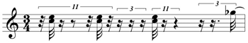
[2.3] This approach works well for the relatively long durations and sparse texture of the opening and closing sections of Study 33. As the density of events increases and durations become smaller, however, this approach is no longer successful, since there are limits to how finely we can subdivide. Thus, for most of the study, Usher uses a different technique that can be clearly observed in the opening of the third canon of the study (Figure 6). Note the nearly consistent use of 11-tuplets over a quarter note, and triplets that are effectively sextuplets over an eighth note. How did Usher arrive at this approximation of the original? Based on my personal communication with Usher and examination of his rather large spreadsheet of calculations, Usher proceeded in a fairly intuitive manner, seeking simply to place each note as close as possible to its irrational placement in the original. But why these particular tuplets, and why do they often alternate? Keep in mind that tuplets are unnecessary where the notation can be simplified. For example, the violin 2 line in measure 55 could have been notated as in Figure 7. Notating passages in this manner would have made the underlying structure clearer at the expense of making the notation needlessly complicated.
[2.4] The key to realizing irrational tempos is to approximate the ratio with a suitable rational polyrhythm. This is possible because any irrational number can be approximated to any degree of accuracy by rational numbers. For \(\sqrt{2}\), close approximations include \(\frac{7}{5} = 1.4\), \(\frac{10}{7}\approx1.429\), \(\frac{17}{12}\approx1.417\), \(\frac{24}{17}\approx1.412\), \(\frac{41}{29}\approx1.4138\), \(\frac{58}{41}\approx1.4146\), and so on. As the absolute value of the numerator and denominator increase, the approximation comes ever closer to the original irrational number. When deciding which rational approximation to use, the trick is to balance mathematical accuracy with feasibility of performance. A polyrhythm of 41:29 is already much too complicated to realize in performance without the aid of click tracks, so we can throw out \(\frac{41}{29}\) and \(\frac{58}{41}\) as impractical.
[2.5] On the other hand, the ratios \(\frac{7}{5}\) and \(\frac{10}{7}\) may be too simple to create the illusion of an irrational tempo ratio. For any rational tempo ratio there is a higher-level periodicity, what Gann 1995 refers to as the convergence period, which results from the (potential) simultaneous attacks between the voices. For example, in a 7:5 ratio the convergence period contains five beats or pulses in the slower voice and seven beats or pulses in the faster. The shorter this convergence period the easier it is for the listener to perceive, and the perception of any higher-level periodicity between the voices will work against the illusion of irrational tempo ratios, which contain no such convergence periods.
Figure 8. 7:5 tempo ratio with a convergence period of \(\frac{7}{8}\) seconds
(click to enlarge)
Figure 9. Convergence periods for (a) 10:7 tempo ratio, (b) 17:12 tempo ratio, and (c) 24:17 tempo ratio

(click to enlarge)
Figure 10. 5+6+6 division in the tempo ratio \(\frac{24}{17}\)

(click to enlarge)
Figure 11. 11+6 division in the tempo ratio \(\frac{24}{17}\)

(click to enlarge)
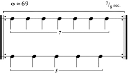
[2.6] Suppose the faster voice in a 7:5 tempo ratio is moving at the rate of eight pulses per second (Figure 8). Then the convergence period will be just \(\frac{7}{8}\) seconds, setting up a readily perceived hypermetric tempo of nearly 69 bpm. If the rhythms are syncopated, as is often the case with Nancarrow, so that the beginning of the period is seldom articulated by both voices, then this convergence period may not be apparent. It depends on the context.
[2.7] Maintaining the same rate of eight pulses per second in the faster voice, a 10:7 ratio yields a convergence period of 1.25 seconds or a hypermetric tempo of 48 bpm (Figure 9a). This is a somewhat larger convergence period, but the hypermetric pulse is still fairly prominent. Tempo ratios of 17:12 (Figure 9b) and 24:17 (Figure 9c) yield noticeably longer convergence periods and slower hypermetric pulses that are more difficult to perceive. In a sense the ratios 17:12 and 24:17 constitute a kind of “sweet spot” for rational approximations of a \(\sqrt{2}\) tempo ratio, not too complex as to be unrealizable (e.g., \(\frac{41}{29}\)), but not too simple that the rational basis of the ratio is readily perceived (e.g., \(\frac{7}{5}\) and \(\frac{10}{7}\)).
[2.8] Even so, dividing a longer time span into 17 equal parts is extremely difficult, especially when various syncopations are involved. For this reason, \(\frac{24}{17}\) is preferable to \(\frac{17}{12}\), since the former places the more difficult subdivision in the slower moving voice. An additional strategy is to approximate this division in the same way that \(\frac{24}{17}\) is an approximation of \(\sqrt{2}\). For example, we could divide 17 as evenly as possible into three groups, yielding a 5+6+6 division (Figure 10).
[2.9] Unfortunately, this solution is unsatisfactory because the convergence period is much shorter and the pulse stream of the slower voice is noticeably uneven. In fact, moving from quintuplet to sextuplet represents a 20% increase in the pulse rate. We can mitigate both of these problems by combining the first two beats into a single 11-tuple, rendering the \(\frac{24}{17}\) polyrhythm as \(\frac{16+8}{11+6}\) (Figure 11). Even though (potentially) simultaneous attacks occur on beats one and three, the overall convergence period remains at three seconds. Additionally, the slower-moving pulse stream is more even, as moving from 11 pulses over two beats to six pulses over one beat (equivalent to twelve pulses over two beats) represents only a 9% increase in the pulse rate. With a variety of rhythmic durations and syncopations this slight unevenness will be extremely difficult to perceive.
[2.10] Now we have a better understanding of how the alternation of 11-tuplets and triplets/sextuplets arose out of Usher’s intuitive approach. Passages in the arrangement that do not strictly alternate between these two types of subdivision typically occur for one of two reasons. Most commonly, an 11:8 polyrhythm has swapped positions with a 6:4 (or 3:2) polyrhythm. For example, measures 59–62 (see Figure 6) contain the following series of polyrhythms in the second violin:
| 11:8 11:8 | 11:8 3:2 3:2 | 11:8 3:2 (implied) | 11:8 3:2 | |
| measure: | 59 | 60 | 61 | 62 |
Simply swapping the third and fourth polyrhythm results in a familiar alternation, yielding the \(\frac{16+8}{11+6}\) polyrhythm starting in the second half of measure 59:
| 11:8 11:8 | 3:2 11:8 3:2 | 11:8 3:2 (implied) | 11:8 3:2 |
[2.11] Occasionally, a single “extra” 11-tuplet, such as at the beginning of measure 59, is necessary to make sure that the voices continue to align properly. For every 24 pulses in the faster voice, at the ratio of \(\sqrt{2}\) there should be just slightly less than 17 pulses in the slower voices (\(\frac{24}{\sqrt{2}} \approx 16.971\)). While this error (0.029) is very small, with each repetition of the polyrhythm the total error accumulates. As the error grows, the pulses of the slower voice progressively drift from where they should be in relation to the faster voice, affecting the vertical alignment of the voices and potentially damaging Nancarrow’s careful harmonic control of the contrapuntal lines. One solution to this problem is to use two approximations of \(\sqrt{2}\); a lower approximation and an upper approximation. A good candidate for an upper approximation is \(\frac{16}{11} = 1.\overline{45}\) (\(\frac{24}{17} < \sqrt{2} < \frac{16}{11}\)), which is relatively close to \(\sqrt{2}\) and is already a component of the \(\frac{16+8}{11+6}\) approximation of \(\frac{24}{17}\). At the ratio of \(\sqrt{2}\), for every 16 pulses in the faster voice there should be slightly more than 11 pulses in the slower voice. Essentially, the slower voice moves too quickly at \(\frac{24}{17}\) and too slowly at \(\frac{16}{11}\), which is why we can use these two ratios to compensate for one another.
3. Four approximations of \(\sqrt{2}\)
Example 1. Opening of canon 3, Nancarrow’s original player-piano study
Example 2. Opening of canon 3, Usher’s arrangement
a. both voices
. b. slower voice only
[3.1] In this section we will compare the opening of canon 3 from Nancarrow’s original Study 33 with four different approximations of this same passage: (1) Usher’s arrangement; (2) a hypothetical example based on approximating ratios using 7:5 and 14:9 as lower and upper approximations; (3) a hypothetical arrangement based on approximating time points; and (4) Nancarrow’s own approximation of this passage in a later section of the original study. Readers may wish to begin by listening to the excerpt from Nancarrow’s original player-piano study, given in Example 1.
[3.2] Example 2 provides audio files of Usher’s arrangement of the opening of canon 3, the score of which is given as Figure 6. Audio files in Example 2 and Figures 12–14 use the same MIDI piano sound in order to facilitate comparison of the approximations with one another.
Figure 12. Hypothetical version of canon 3, approximating tempo ratio

(click to enlarge and listen)
Figure 13. Hypothetical version of canon 3, approximating beat placement

(click to enlarge and listen)
Figure 14. Nancarrow’s approximation of \(\sqrt{2}\), Study No. 33, systems 56–60

(click to enlarge and listen)
[3.3] In the same spirit as Usher’s arrangement, Figure 12 also uses limited rational ratios to approximate \(\sqrt{2}\). In this case, the lower and upper ratios are 7:5 and 14:9, respectively. Despite the use of simpler ratios, this is a very convincing approximation due in part to the syncopated rhythmic figures and the fact that there are no simultaneous attacks on the beat.
[3.4] Figure 13 presents a different hypothetical approximation, one that uses many different subdivisions to approximate beat placement rather than tempo ratio. The goal of this approach is to minimize deviations of time points between the original and its approximated version. The main problems with this approach are that (1) the use of many different subdivisions can make performance more difficult, and (2) the approximated voice can often sound uneven, hindering the perception of a steady tempo and tempo ratio. This unevenness can be heard in the single-voice audio file in the Audio files in Figure 13.
[3.5] Finally, Nancarrow provides his own approximation of \(\sqrt{2}\) in the process of recalling and developing canon 3 within the much larger fourth and final canon. At the point where canon 3 is recalled (system 56), both voices of the canon are given to the top voice (see Figure 14). While Nancarrow could have preserved the original \(\sqrt{2}\) tempo ratio, he chose to round the attack points of the lower part to the nearest sixteenth note (for the most part). Specifically, durations between attack points in the upper part are approximated in the lower part in the follow manner:
| Upper part (sixteenths) | Lower part (sixteenths) | \(2:\sqrt{2}\) ratio |
| 4 | 5 | \(4\sqrt{2} \approx 5.66\) |
| 8 | 11, 12, or 13 | \(8\sqrt{2} \approx 11.31\) |
| 12 | 17 | \(12\sqrt{2} \approx 16.97\) |
| 16 | 23 or 24 | \(16\sqrt{2} \approx 22.63\) |
The alternate approximations in the table above give Nancarrow the flexibility to ensure that the lower part does not drift too far from where it would be in a precise \(\sqrt{2}\) ratio. This approximated recollection is like a strange version of canon 3, one in which all traces of irrationality have been removed and yet the tempo ratio is perceived as roughly the same and the alignment of events between the two parts is undisturbed.
4. Convergence points
[4.1] One of the biggest challenges in realizing irrational tempo canons for human performance is the placement of convergence points. These are moments of time in which multiple voices moving in different tempos converge on the same position in the canon line, where the echo distance is zero. (The echo distance is “the temporal gap between an event in one voice and its corresponding recurrence in another” [Gann 1995].) Since the echo distance between canonic voices in different tempos is always increasing or decreasing, tempo canons are always either moving toward or away from a convergence point. The structural properties of a tempo canon are thus determined in large part by the placements of these convergences (see Scrivener 2002 for more on the structural significance of convergence points in Nancarrow’s tempo canons).
Figure 15. (a) Converging-diverging canon, (b) Diverging-converging canon, and (c) Abstract canonic structure of Study 33

(click to enlarge)
Figure 16. Tempo exchange, canon 1, Nancarrow
(click to enlarge)
[4.2] There are two different types of tempo canons found in Study 33 (see the structural diagrams in Figure 15). The first is a converging-diverging canon, in which the voices (indicated by horizontal lines) enter staggered from slower to faster, move toward a central convergence point (indicated by vertical lines), and then recede from this point, thus ending in the reverse order of their entrance (Figure 15a). The second type is a diverging-converging canon, featuring convergence points at the beginning and end and a tempo exchange (indicated by diagonal, crossing lines) at or very near the midpoint of the canon (Figure 15b).(1) Before this tempo exchange, the voices diverge from the initial convergence point with the faster voice moving ahead of the slower voice; at the tempo exchange the faster voice becomes the slower and vice versa; after this exchange the voices converge toward the ending convergence with the faster voice catching up to the slower. Study 33 consists of four canons: canons 1 and 3 are of the second type; canon 2 is the first type; the final canon, canon 4 (by far the longest), is a combination of both types with a converging-diverging-converging pattern (Figure 15c). In order to have a better understanding of the problems that arise, we can look at Usher’s solution to the two types of canons separately.
[4.3] The problem with the diverging-converging type of tempo canon is the realization of the tempo exchange in the middle of the canon. Specifically, if the tempo ratio is irrational, then the voices cannot change tempo at the same time. For example, in canon 1 each voice has 27 (whole-note) beats at the faster tempo and 19 beats at the slower tempo. Since the ratio of these beats, 27:19, is a close approximation of \(\sqrt{2}\), each voice will switch tempos near but not precisely at the midpoint of the canon. In particular, 19 beats at the slower tempo is only \(19\sqrt{2} \approx 26\frac{7}{8}\) beats at the faster tempo, leaving what we might term an exchange gap of \(\frac{1}{8}\) beats (Figure 16).
[4.4] For his arrangement Usher had to choose between switching tempos at 27 or \(26\frac{7}{8}\) (quarter-note) beats of the faster voice. Choosing the former results in bar lines after the tempo exchange that do not align with the faster voice (Figure 17). Choosing the latter amounts to dropping an eighth of a beat (a 32nd note in this case), yielding a much simpler rhythmic notation after the exchange (Figure 18). Usher’s arrangement surrounding the midpoint of canon 1 is shown in Figure 19. The tuplets signal the exchange of tempos, switching from the lower voice before measure 12 to the upper voice in measure 13 (tuplets always being associated with the slower moving voice). The use of the \(11\atop32\) time signature allows the bars to line up with the change of tempo in the lower voice.
Figure 17. Realization of the tempo exchange in canon 1 that yields an unnecessarily complex rhythmic notation after the exchange
(click to enlarge) Figure 19. Tempo exchange, canon 1, Usher
(click to enlarge) | Figure 18. A different realization of the same tempo exchange that yields a much simpler rhythmic notation
(click to enlarge) Figure 20. Tempo exchange, canon 3, Nancarrow
(click to enlarge) |


Figure 21. Tempo exchange, canon 3, Usher

(click to enlarge)
Figure 22. Tempo exchange, canon 4, Nancarrow
(click to enlarge)
[4.5] The tempo exchange in canon 3 is much simpler to realize. In this canon, there are 147 quarter notes in the faster tempo and 104 quarter notes in the slower tempo prior to the tempo exchange. Because \(\frac{147}{104}\) is an extremely close approximation of \(\sqrt{2}\) (\(|\frac{147}{104} - \sqrt{2}| \approx .0008\)), tempo changes in each voice are only 17 ms apart and can be treated for all practical purposes as simultaneous (Figure 20). In the relevant passage from Usher’s arrangement, we can see that the tempo exchange happens simultaneously in both voices, the fourth eighth-note of measure 75 marking the exchange without any adjustments necessitating an awkward time signature (Figure 21).
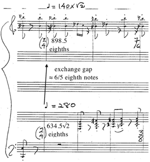
[4.6] The tempo exchange in canon 4 is by far the messiest. In Nancarrow’s study, there are \(898\frac{1}{2}\) and \(634\frac{1}{2}\) eighth notes, respectively, in the faster and slower tempos. As expected, this ratio of beats (\(\frac{1757}{1269}\)) is a very close approximation of \(\sqrt{2}\). However, \(634\frac{1}{2}\) beats at the slower tempo is roughly equal to only \(634\frac{1}{2}\sqrt{2} \approx 897.3\) eighth notes at the faster tempo, roughly \(\frac{6}{5}\) of an eighth note (or \(\frac{3}{5}\) of a quarter note) less than \(898\frac{1}{2}\) (Figure 22). While this may seem like a very small amount, at the notated tempo of Usher’s arrangement (quarter note equals 64) \(\frac{6}{5}\) of a thirty-second note is around 140 ms, a discrepancy that Usher chooses to avoid. Instead of dropping \(\frac{6}{5}\) thirty-seconds from a measure, he inserts an additional measure of \(\frac{4}{5}\) thirty-seconds (yielding a time signature of \(\frac{4}{5}\times\frac{1}{32}=\frac{1}{40}\)) to accomplish the same thing—aligning the following bar with the tempo change in the lower voice (Figure 23).
Figure 23. Tempo exchange, canon 4, Usher
(click to enlarge) | Figure 24. Opening of canon 2, Nancarrow
(click to enlarge) |
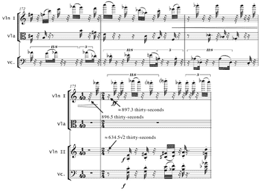

Figure 25. Opening of canon 2, Usher

(click to enlarge)
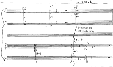
[4.7] The problem with the converging-diverging type of canon is notating the correct duration of the slower voice prior to the entrance of the faster voice. With irrational ratios this typically necessitates awkward partial measures. For example, in canon 2 of the original study the faster voice enters after four whole notes in the slower tempo and one half note in the faster tempo for a total duration of \(4\sqrt{2} + \frac{1}{2} \approx 6\frac{1}{6}\) whole notes in the faster tempo (Figure 24). The actual notated duration in Usher’s arrangement (taking into account that Usher’s quarter notes are equivalent to Nancarrow’s whole notes) is very close, \(6\frac{1}{10}\) quarters, necessitating a \(3\atop20\) measure that is equivalent to \(\frac{3}{5}\) of a quarter note. Alternatively, an initial \(1\atop6\) measure would give the precise \(6\frac{1}{6}\) quarter-note duration (Figure 25).
[4.8] In the initial convergence of canon 4 of the original study, both voices have 79 quarter notes prior to the convergence point, each at their respective tempo. The upper voice thus begins \(79\sqrt{2} - 79 \approx 32\frac{2}{3}\) quarter notes, or \(8\frac{1}{6}\) half notes or \(2\frac{1}{24}\) whole notes prior to the entrance of the lower voice (Figure 26). In the relevant passage from Usher’s arrangement we find that the upper voice enters after the lower voice by precisely this duration—four bars of \(2\atop4\) plus an additional bar of \(1\atop24\) (or \(\frac{1}{6}\) of a quarter note) (Figure 27).
Figure 26. Opening of canon 4, Nancarrow
(click to enlarge and see the rest) | Figure 27. Opening of canon 4, Usher
(click to enlarge) |


5. Arditti Quartet’s performance
Figure 28. Opening of canon 3 with Arditti String Quartet recording

(click to enlarge, see the rest, and listen)
Figure 29. Graph of beats with respect to time and the resulting trend lines in the recording of the opening of canon 3

(click to enlarge)
[5.1] Finally, we turn to a brief analysis of the Arditti Quartet’s 2007 recording of Usher’s arrangement, focusing on the first half of canon 3. (Figure 28 reproduces the opening of canon 3 with an excerpt from the Arditti’s recording.) All of the mathematical and notational precision would be pointless if the Arditti was not capable of rendering the rhythmic intricacies with sufficient accuracy. However, we should not be concerned with accuracy for its own sake. Instead, what matters is if the performance of the arrangement is close enough to be perceived as a reasonable facsimile of the original player-piano study. Thus, the two important questions are:
- Is each voice perceived as moving in a steady tempo and are these perceived tempos in roughly the right ratio?
- Do the events occur at roughly the right time and, most importantly, is the order of events preserved?
[5.2] Figure 29 plots attack points for both voices (first and second violins) in the first half of canon 3 with beats measured in eighth notes from the beginning of the canon along the vertical axis and time measured in seconds along the horizontal axis. Superimposed on each of these voice plots are their corresponding linear trend lines. The slope of the trend lines corresponds to the central tempo of each voice, with \(\approx 116.1\) bpm in the first violin and \(\approx 82.18\) in the second violin, giving a tempo ratio (\(\approx 1.413\)) that is very close to \(\sqrt{2}\). As can be seen on the figure, the plots for both voices are fairly straight and conform closely to the trend lines. This tight fit between the attack points and their trend lines corresponds to a reasonably steady tempo. Usually, kinks in the line result from a single note beginning uncharacteristically early or late, after which the plot returns to the trend line.
[5.3] The closer the actual timings are to the underlying tempo the stronger the perception of a steady tempo. Measuring timings for the first and second violins against the trend lines in Figure 20 yields average absolute deviations of 73 and 77 milliseconds, respectively. However, since the underlying tempo will naturally vary slightly over the course of the half-minute excerpt, it is better to measure deviations against trend lines based on shorter regions. Using regions of \(\pm 2\) attack points for each attack yields average absolute deviations of 29 and 47 milliseconds, respectively, for the first and second violins.
Figure 30. Inter-onset intervals in the original and recorded versions of the opening of canon 3
(click to enlarge)
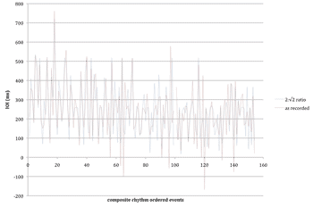
[5.4] Figure 29 would seem to answer the first question in the affirmative, which certainly corresponds to my hearing—onsets within each voice give a strong impression of steady tempos in approximately the right ratio. The second question essentially concerns the relation of onsets between the two voices. One way to answer this question is to compare the composite rhythm of the original study with the composite of the recording. Figure 30 plots the inter-onset-intervals (IOIs) for the composite rhythm of the original player-piano study in blue. (Timings have been adjusted to match the actual tempo of the recording rather than the notated tempos of Nancarrow’s study or Usher’s arrangement.) The first IOI, spanning from the first onset in the upper voice of canon 3 to the first onset in the lower voice, is 107 ms; the second IOI, spanning from the first onset in the lower voice to the second onset in the upper voice, is 410 ms; and so forth. The IOIs for the composite rhythm of the recording are plotted in red. The better the fit between these two plots, the more accurate is each player’s beat placement with respect to the other part. The correlation between the original and recorded composite rhythms is \(r=.77\), and the average absolute deviation is 67 ms. This suggests that the alignment of the parts is relatively accurate, though there is a certain amount of error as well.
[5.5] However, relatively small inaccuracies are not particularly important or even audible in this context. Indeed, a large part of the charm of irrational tempo ratios is that it is impossible to reconcile the alignment of the individual parts, since their composite rhythm is also irrational. More important are the few IOIs in Figure 29 that are negative. For any two successive onsets, \(t_1\) and \(t_2\), the IOI is simply \(t_2 - t_1\). A negative IOI thus implies that \(t_2\) occurs before \(t_1\), a situation that does not preserve the ordering of events in the original study. These “event swaps” are potentially more noticeable than other deviations that nonetheless preserve the original event ordering. Here are the timing details (measured in milliseconds) for each of the six event swaps (the swaps are marked on the score in Figure 28):
| event swap | IOIs (original) | IOIs (recorded) |
| 1 | 75 | \(-\)44 |
| 2 | 139 | \(-\)100 |
| 3 | 106 | \(-\)57 |
| 4 | 53 | \(-\)168 |
| 5 | 72 | \(-\)16 |
| 6 | 91 | \(-\)76 |
To put these swaps in perspective, at the performance tempo of approximately 58 quarter notes per minute, a single sixteenth-note triplet is 172 ms in duration. Thus, all six swaps involve events that are already very close together in the original study. As one example, the second (and largest) swap results from the event in the first violin beginning the equivalent of a quintuplet thirty-second after the event in the second violin, instead of beginning before by roughly a thirty-second. All in all, these event swaps and other discrepancies between the recording and the original score are entirely inconsequential.
Figure 31. (a) First violin measure 68 as performed and (b) as notated

(click to enlarge)
[5.6], There is a seventh event swap, indicated in Figure 28 by a dashed arrow, which arises for a different reason than the other six swaps. In the recording, the first violin plays measure 68 as shown in Figure 31a, rather than as notated (Figure 31b). (I have simplified the notated rhythms to make the nature of the discrepancy clearer.) Thus, this event swap results from an alteration of the basic rhythmic category rather than from issues of microtiming (Clarke 1999). My purpose is not to critique the Arditti Quartet’s recording; as recorded, the rhythmic figure is more in keeping with the rest of canon 3. More to the point, I find it telling that the most noticeable discrepancy between recording and score has nothing to do with the formidable rhythmic complications of approximating irrational rhythmic ratios. Indeed, it speaks to the Arditti’s ability to meet seemingly impossible challenges as well as to Usher’s ingenuity in arranging an irrational tempo canon for live string quartet.(2)
Clifton Callender
Florida State University
Tallahassee, FL 32303
clifton.callender@fsu.edu
Works Cited
Callender, Clifton. 2001. “Formalized Accelerando: An Extension of Rhythmic Techniques in Nancarrow’s Acceleration Canons.” Perspectives of New Music 39, no. 1: 188–210.
Clarke, Eric. 1999. “Rhythm and Timing in Music.” In The Psychology of Music, edited by D. Deutsch. San Diego: Academic Press.
Fürst-Heidtmann, Monika. 2012. “Dated and annotated list of works, premiers and arrangements of the music of Conlon Nancarrow” (accessed August 26, 2012).
Gann, Kyle. 1995. The Music of Conlon Nancarrow. Cambridge University Press.
—————. 2012. “Conlon Nancarrow: Annotated List of Works” (accessed August 26, 2012).
Hocker, Jürgen. 2012. “List of Works English Version” (accessed August 26, 2012).
London Sinfonietta. 2012. “Impossible Brilliance: the music of Conlon Nancarrow” (accessed August 26, 2012).
Scrivener, Julie. 2002. “Representations of Time and Space in the Player Piano Studies of Conlon Nancarrow.” PhD diss., Michigan State University.
Thomas, Margaret. 1996. “Conlon Nancarrow’s ‘Temporal Dissonance’: Rhythmic and Textural Stratification in the Studies for Player Piano.” PhD diss., Yale University.
Arditti Quartet. 2007. Quartets and Studies. Mainz: Wergo. CD.
Bugallo-Williams Piano Duo (Helena Bugallo and Amy Williams). 2004. Conlon Nancarrow: Studies and Solos. Mainz: Wergo. CD.
Ensemble Modern. 1993. Conlon Nancarrow Studies: arr. Yvar Mikhashoff. Frankfurt: BMG Music. CD.
London Sinfonietta. 2011. Adès In Seven Days / Nancarrow Studies Nos. 6 & 7. Signum Records. CD.
Footnotes
1. Thomas 1996 categorizes tempo canons into four structural types: converging, diverging, converging-diverging, and diverging-converging.
Return to text
2. My thanks to Evan Jones for his valuable feedback, Helena Bugallo for discussing her arrangement of Study No. 19, and Paul Usher for his willingness to answer questions and provide materials related to his work on the arrangement. Earlier versions of this paper were presented at the 2013 Music Theory Southeast Conference and published as part of an online symposium, Conlon Nancarrow, Life and Music, at http://conlonnancarrow.org/symposium/papers/callender/irrational.html.
Return to text
Copyright Statement
Copyright © 2014 by the Society for Music Theory. All rights reserved.
[1] Copyrights for individual items published in Music Theory Online (MTO) are held by their authors. Items appearing in MTO may be saved and stored in electronic or paper form, and may be shared among individuals for purposes of scholarly research or discussion, but may not be republished in any form, electronic or print, without prior, written permission from the author(s), and advance notification of the editors of MTO.
[2] Any redistributed form of items published in MTO must include the following information in a form appropriate to the medium in which the items are to appear:
This item appeared in Music Theory Online in Volume 20, Issue 1 in March 2014. It was authored by Clifton Callender (clifton.callender@fsu.edu), with whose written permission it is reprinted here.
[3] Libraries may archive issues of MTO in electronic or paper form for public access so long as each issue is stored in its entirety, and no access fee is charged. Exceptions to these requirements must be approved in writing by the editors of MTO, who will act in accordance with the decisions of the Society for Music Theory.
This document and all portions thereof are protected by U.S. and international copyright laws. Material contained herein may be copied and/or distributed for research purposes only.
Prepared by Michael McClimon, Editorial assistant
Number of visits:
21612