Reconsidering Klumpenhouwer Networks

Michael H. Buchler
KEYWORDS: Klumpenhouwer networks, transformation, recursion, pitch class, criticism
ABSTRACT: This article raises concerns about Klumpenhouwer networks (K-nets) and their analytical deployment. The critique is structured around four central issues: K-nets as dual transformations, relational abundance (so-called “promiscuity”), phenomenology, and the role of recursive hierarchies. In the article’s initial section, Shaugn O’Donnell’s dual transformation model will be promoted as an equivalent and more facile substitute for K-nets in most situations. The second section, on relational abundance, discusses the double-edged sword of transformational flexibility: as attractive as it may be to associate sets that are not simple canonical transforms of each other, the manner in which some analysts use K-nets—and especially K-net families—seems to open a Pandora’s Box of relational permissiveness. The section on phenomenology raises questions of perceptibility, particularly with regard to negative isography. Finally, the section on recursion examines the musical and structural commensurability of deep- and surface-level networks.
Copyright © 2007 Society for Music Theory
[1] This article critically examines both Klumpenhouwer networks (K-nets) and their analytical deployment. Since David Lewin’s introductory article in 1990, K-nets have been among the most frequently discussed and analytically utilized tools for post-tonal transformational analysis.(1) Because they increasingly form the methodological basis for post-tonal scholarship—including entire issues of Music Theory Spectrum and Intégral devoted to their theoretical elaborations and analytical functionality—it seems right to consider (or reconsider) the sorts of information they are best able to convey and also to scrutinize their music-analytical use.
[2] K-nets are elegant structures that not only allow us to relate pitch-class sets (pcsets) in multiple ways, but facilitate hierarchical structures in which individual chords are shown to be comparable to networks of chords, networks of networks, and so forth.(2) To many proponents, this potential for “recursive” relations serves as the K-nets’ raison d’être. I believe—and hope to demonstrate—that such hierarchies might just as easily be considered their greatest pitfall. K-nets also enable us to relate sets and networks that are neither transpositionally nor inversionally equivalent, but this is another double-edged sword: as nice as it is to associate similar sets that are not simple canonical transforms of one another, the manner in which K-nets accomplish this arguably lifts the lid off a Pandora’s Box of relational permissiveness. Clearly, the more ways that it is possible to draw equivalent relations, the less significant those relations become.
[3] Beyond the question of significance, when data can be shaped in multiple ways, we necessarily rely upon some mode(s) of interpretation to form and arrange our analytical objects. While interpretation lies (or arguably ought to lie) at the heart of music analyses, I will suggest that problems can arise when there is too great an abundance of data to sift, when we do not have a clear idea of how to sift, when we have not adequately negotiated the boundaries of our data set, when some interpretations are represented as taxonomical prototypes, and when a priori extramusical assumptions begin to drive our analytical choices. The first and longest part of this essay examines K-net structure (apart from its implementation); the remainder amounts to a detailed editorial on associated theoretical and interpretive matters. More specifically, the following four broad topics will be addressed:
- K-nets as dual transformations;
- The issue of relational abundance (“promiscuity”);
- The phenomenology of displaced pitch-class inversion and dual inversion;
- The issue of hierarchy and recursion.(3)
[4] Topics III and IV (phenomenology and recursion) were raised lucidly and succinctly by Joseph Straus during the closing plenary session at the 2003 Mannes Institute on Transformational Theory. Regarding recursion, Straus commented that it “is only a problem when our desire for it leads us to emphasize musical features that might otherwise be of relatively little interest.” Straus was more skeptical about dual inversion, noting that as pc-space constructions they are difficult, if not impossible, to hear when realized and concluding that they “have no intrinsic interest, they correspond to no musical intuitions, they provide an answer to a question that no one has cared to ask.”(4) This present essay will briefly expand upon Straus’s comments regarding phenomenology, and will present a broader case against the analytical use of recursion.(5)
I. K-Nets as Dual Transformations
[5] Like a host of other tools, including similarity relations, split or near transformations, and topographical distance metrics, Klumpenhouwer networks allow us to relate two objects that belong to different taxonomical classes. Those “objects” have generally been pitch-class sets (pcsets), though other musical types could be used. In particular, K-nets and dual transformations both describe situations where some of the notes in a pcset are transformed in one way while the other notes are transformed in some other way. From K-nets’ outward appearance as unified networks of nodes and arrows, this dual transformational basis might not be so evident; this section teases it out.
[6] K-nets always integrate some combination of transpositional and inversional relationships, denoted by the node-traversing arrows or line segments, respectively. The way we associate K-nets is through isography. If their graphs look the same in some well-defined respects, they are related. The standard definition of K-net isography goes something like this: two networks are considered isographic if they have the same configuration of nodes and arrows and if their respective Tn arrows either carry the same values of n or if those values are inversely related. Also, the respective In values must either differ by or sum to a constant integer, depending upon whether we are showing positive or negative isography.
[7] But one can get at the information conveyed by isography, particularly the hyper network transformations, without using I-arrows at all. To illustrate that point, it will be helpful to review the basic structural characteristics of K-nets. I will attempt to do so as plainly as possible through six essential statements (S1 through S6) that describe normative K-net usage. These six statements together with their accompanying commentary might serve as a primer on both K-net rudiments and K-net practice. The first three statements describe K-net construction; the last three deal with isography, the basic method for comparing network structures. Along the way, I will suggest a simpler analytical organization—based upon the dual-transformation model—that whittles away those portions of K-net structures that are not vital to their use. I will simultaneously advocate one way to convey more valuable information without altering fundamental K-net structures. My central goal here is to draw out the intuitive basis of K-nets, and to use the same data that goes into shaping their relations to convey clearer and more meaningful musical connections.
|
[8] S1 |
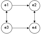
Figure 1. A network of nodes and arrows
(click to enlarge) A network is formed of nodes and arrows. Nodes depict elements; arrows depict relationships among the elements. Arrows can be bi-directional, indicating an involutional relationship (e.g., inversion), or they can be unidirectional, indicating a non-involutional relationship (e.g., transposition). Figure 1 shows a visual network representation. Comment 1.1: “Elements” can signify almost any musical feature, but most often they represent pitch classes or networks of pitch classes. All elements within a single network must represent the same class of objects (all pitch classes, all networks, etc.). K-net analysis often relies heavily on the ability to show identical-looking K-nets that operate on different classes of objects. Such K-net “recursion” (mentioned informally earlier) will be discussed in the final section of this article. Comment 1.2: I chose the broader and more neutral term “relationships” rather than “transformations” because of the latter’s stronger metaphorical implications—of actively mapping one thing onto another. As I will show, these devices can be constructed in a non-transformational (metaphorically ‘static’) or a less strictly transformational manner. Like elements, relationships can theoretically take a wide variety of forms (c.f., Lewin 1987), but in practice they have most always been limited to transposition and inversion. Comment 1.3: In his later work, Lewin used simple line segments (with no arrow heads) in place of bi-directional arrows. We will henceforth adopt that practice in this article. |
|
[9] S2 |
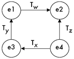
Figure 2. An abstract four-node K-net model
(click to enlarge) Figure 3. An abstract four-node T-net
(click to enlarge) Figure 4. Two four-node I-nets (that are really K-nets)
(click to enlarge and see the rest) K-nets employ combinations of transposition and inversion operators.(6)At least two pairs of elements must not be connected by transposition (Tn arrow). Figure 2 shows an abstract four-node K-net model.
Comment 2.1: Following Lewin’s convention, I will use the notation Tn for transposition by n semitones and In
for the inversion that exchanges any two pitch classes that sum to n mod 12. Since inversion is an involution (if In(p) Comment 2.2: At least two pairs of elements must be transpositionally disconnected because if a fully connected network contained only a single In arrow, it would essentially be a T-network (i.e., a network of nodes connected entirely by Tn arrows).(7)Imagine a network with nodes a, b, and c. If the distance between a and b is known to be Tx and the distance between b and c is known to be Ty, then elements a and c are clearly, if implicitly, related by Tx+y, not by some inversion. Were the nodes of a network connected entirely via transposition arrows (i.e., a T-net), then the intervals separating each pair of nodes would be fixed. Such a network is shown in Figure 3. T-nets do little more than describe transpositionally defined set classes (Tn classes). Since Tn classes are well understood and easily defined, using a more complex system to generate the same result would serve no purpose, at least at the level of pitch class. In Figure 3, we could omit any one of the arrows without effectively losing information. For example, if we removed the Tz arrow, it would still be clear that the relationship between e4 and e2 is Tx+y+w. Indeed, this happens to be true for K-nets as well; a missing T-arrow can be inferred by the difference between the I-arrows. This matter of acknowledging implicit network transformations will arise again later. Comment 2.3: We do not need to discuss networks that are connected entirely via inversion arrows (we might call these “I-nets”) because they are fundamentally indistinct from K-nets. An informal proof is shown below:
|
[10] S3 |
Every node is graphically connected (by arrows) to at least two other nodes in the network. Comment 3.1: These connections are merely the ones displayed. As just demonstrated in Comment 2.3, every element at least implicitly connects to every other element in the network through the transitivity of transposition and inversion operators. One only need display as many connections as are necessary to implicitly establish the relationship between every pair of nodes. If, in Figure 2, the arrow between e1 and e2 were
erased, we would still know how e1 and e2 are related by virtue of
the other arrows. Moving counterclockwise from e1, we see that e1 is
related to e2 by IyTxIz (reading left to right). Since e3 = Iy(e1) is equivalent to e3 =
y-e1 and the expression e4 = Tx(e3) is equivalent to e4 = e3+x, we can say that the relationship between e1 and e2 is modeled by: TxTy = Tx+y IxIy = Ty-x TxIy = Iy-x IxTy = Ix+y To reflect K-net essentials rather than general K-net practice, we might profitably rewrite S3 as follows: |
[11] S3a |
The relationship between every pair of nodes must be implicit from the network design. Comment 3.2: This understanding of K-net well-formedness accommodates incomplete-looking network structures. It also underscores an important point that is often either overlooked or underemphasized in K-net practice: every node in a K-net must be completely connected within the structure; the arrows merely reflect those relationships upon which we choose to focus. Consequently, K-net isography (and K-net analysis) requires picking and choosing those facets of a chord that we want to compare.(8) Isography therefore differs from devices such as equivalence or similarity measures (which generally do not cherry pick among intervals or subsets to compare) and also from other transformational devices that show mappings of one set onto another. In Section IV (on relational abundance), I will argue that this flexibility can be cast either as a feature or a potential pitfall. |
[12] S4 |
Particular K-net interpretations are not directly compared; rather, it is their graphs that are compared. Graphs that are structurally equivalent are said to be “isographic.” There are two ways that isography may be attained: positively isographic networks have the same transposition (Tn) arrows; negatively isographic networks have inversely related Tn arrows. (The inverse of Tx is T12-x.) Comment 4.1: K-net aficionados may notice and perhaps protest that I have omitted a seemingly fundamental aspect of positive and negative isography.
S4 only mentions that the transpositional relationships are the same in each set; it says nothing about the inversional relations. This is because, as I shall demonstrate, the inversional axes (In arrows) are effectively irrelevant to determining whether isography can be drawn.(9)
We might append the following corollaries to S4:
|
[13] S5 |
“Strong isography” is a special case of positive isography. Two K-nets are said to be “strongly isographic” if they are positively isographic and their respective In arrows are also identical. |
[14] S6 |
The transformation between K-nets (so-called “hyper” transformation) is calculated and expressed as follows:
|
[15] In Comment 4.1, I claimed that network-internal In values are unnecessary to determine whether two K-nets are isographic. Presently, I will show that they are also unnecessary for calculating the exact transformation between K-nets. In other words, I will present a different and simpler way of formulating K-net transformations. Although there is no lack of clarity in Lewin’s and Klumpenhouwer’s definitions of K-nets and network isography (summarized in S6), I find it helpful to conceive of this apparatus in less formal and also rather different terms. So we do not get lost in a sea of definitions and redefinitions, let us momentary step back and recall the conditions under which people turn to K-nets and network isography. The following synopsis might be helpful:
At the basic level of pitch-class relations, K-net isography portrays situations where two sets are each split into a pair of transpositionally defined subsets, and the subsets of one set can be transposed or inverted onto the subsets of the other set.
[16] Imagine Tn arrows as a sort of glue that binds the tones they traverse into Tn-defined set classes. As mentioned in comment 3.2, if we have elements a, b, and c, where b = Tx(a) and c = Ty(b), then it would be gratuitous to draw an arrow from a to c, since, by transitivity, we already know that relation to be Tx+y. When two or more nodes are bound together by Tn arrows, I will collectively refer to them as a “T-set.” A K-net could be redefined as a pair of T-sets that are separated by a particular axis of inversion (as one can infer from comment 2.3 above). So, a three-node K-net will always feature a dyadic T-set and a singleton (even a single note is a T-set by virtue of the implicit T0 relationship to itself). Four-node K-nets can either be split into #3 + #1 T-sets or #2 + #2 T-sets (#n refers to a set of cardinality n), and so forth.(12)
[17] Incidentally, if a K-net is defined as a network of nodes that are completely connected (at least implicitly) by T- and I-arrows, then it will always yield two and only two distinct T-sets. An informal proof of this is simple enough. We know that transposing transpositions yields transpositions; inverting transpositions (or vise versa) yields inversions; and inverting inversions yields transpositions. Any network members not connected by transposition are therefore connected by inversion. Were there three constituent T-sets, A, B, and C, such that In(A)
![]() B and Im(B)
B and Im(B)
![]() C, we would know that members of A and C properly belong to the same T-set because InIm = Tm-n. This is why there can only be
as many as two T-sets. We know that there must be at least two T-sets because if all nodes were transpositionally connected, the resulting structure would be a T-net, not a K-net.
C, we would know that members of A and C properly belong to the same T-set because InIm = Tm-n. This is why there can only be
as many as two T-sets. We know that there must be at least two T-sets because if all nodes were transpositionally connected, the resulting structure would be a T-net, not a K-net.
[18] To determine the mapping from one K-net to another, there is no need to know the inversional axes that connect each network’s two constituent T-sets. Assume two collections X and Y have been interpreted as K-nets such that Tp maps T-set1 of X onto T-set1 of Y. Likewise, Tq maps T-set2 of X onto its partner in Y. More formally: Tp(T-set1(X))
![]() T-set1(Y) and Tq(T-set2(X))
T-set1(Y) and Tq(T-set2(X))
![]() T-set2(Y). The Klumpenhouwer (hyper) transform from X to Y simply equals <Tp+q>, the sum of the split transpositions. In the case of negative isography, we interpret two K-nets such that Ip(T-set1(X))
T-set2(Y). The Klumpenhouwer (hyper) transform from X to Y simply equals <Tp+q>, the sum of the split transpositions. In the case of negative isography, we interpret two K-nets such that Ip(T-set1(X))
![]() T-set1(Y) and Iq(T-set2(X))
T-set1(Y) and Iq(T-set2(X))
![]() T-set2(Y). The Klumpenhouwer transform from X to Y now equals to <Ip+q>, the sum of the split inversions.(13)
T-set2(Y). The Klumpenhouwer transform from X to Y now equals to <Ip+q>, the sum of the split inversions.(13)
[19] Figure 5 demonstrates the transformation from some set X to some set Y both as a split transposition and as normally realized K-nets where the In relations form the basis for comparison. Figure 6 similarly presents two ways of determining negative isography.(14) Focusing on T-set transformations does not merely save time, it also presents a simpler musical scenario: hearing or envisioning dual transpositions or inversions versus hearing or envisioning the differences between multiple dual pc inversions operating simultaneously on each individual collection.
|
Figure 5. Two ways to calculate K-net positive isography
(click to enlarge) |
Figure 6. Two ways to calculate K-net negative isography
(click to enlarge) |
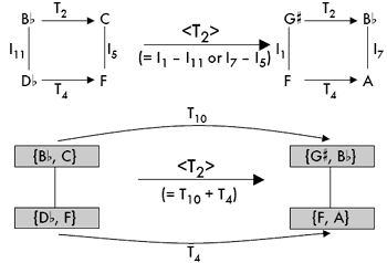

Figure 7. Lewin’s rather large K-net (Figure 1.3 from Lewin 2002)
(click to enlarge)
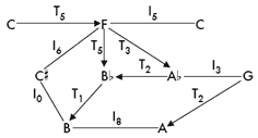
[20] For a more dramatic example of how one might recast K-nets as split transpositions or inversions, let us re-examine what might well be the most elaborate K-net in print. In Lewin’s contribution to Spectrum’s 2002 K-net special issue, he demonstrated that “any K-net, no matter how complex, can be embedded as a contiguous subnetwork of some PL-cycle [Perle-Lansky cycle].” Lewin’s aim (to show the cyclic nature of K-nets and to formalize an interesting claim made by Perle) differs from mine, but en route to making his point, he incidentally demonstrates that any K-net can be cast as a pair of T-sets. For our current purposes, we do not need to delve into the more rigorous demands and formalisms of PL-cycles, but it is worth retracing some of Lewin’s steps before steering onto our own (far more modest) course. The network Lewin produces in his Figure 1.3 is shown here as Figure 7.
[21] If we can draw a path of Tn arrows, we can say that all pcs that lie along that path collectively form a T-set. Figure 8 shows one clear path in Lewin’s network. We must now determine whether each of the remaining pcs can either indirectly be attached to the initial T-set, or whether they collectively or partially form a second T-set. The following discussion will seem more lucid if read while examining Figure 9. A T2 arrow connects, and thereby groups, pcs G and A. Because a path that features two consecutive In arrows implicitly yields a Tn arrow from the first to the third pc, we can connect C![]() to A with a T8 arrow by following the path <C
to A with a T8 arrow by following the path <C![]() — I0 — B — I8 — A>. Connecting the upper-right C is only a bit more complex. F and A
— I0 — B — I8 — A>. Connecting the upper-right C is only a bit more complex. F and A![]() are transpositionally connected as part of the first T-set. The upper-right C is inversionally connected to F. Think of F, A
are transpositionally connected as part of the first T-set. The upper-right C is inversionally connected to F. Think of F, A![]() , and C as forming an incompletely drawn three-note K-net. Every three-note K-net has one and only one Tn arrow; the other notes are connected by inversion. That means that we can envision an implicit I8 arrow between C and A
, and C as forming an incompletely drawn three-note K-net. Every three-note K-net has one and only one Tn arrow; the other notes are connected by inversion. That means that we can envision an implicit I8 arrow between C and A![]() . The transpositional (T5) connection between G and C is now clarified by following the path <G — I3 — A
. The transpositional (T5) connection between G and C is now clarified by following the path <G — I3 — A![]() — I8 — C>. At this point, it is apparent that C
— I8 — C>. At this point, it is apparent that C![]() , A, G, and C cluster to form the other T-set. Like all discrete pairs of T-sets, there are no Tn arrows that can implicitly connect any pc in one T-set to any pc in the other.(15)
, A, G, and C cluster to form the other T-set. Like all discrete pairs of T-sets, there are no Tn arrows that can implicitly connect any pc in one T-set to any pc in the other.(15)
|
Figure 8. One T-set that falls out of Lewin’s rather large K-net
(click to enlarge) |
Figure 9. The other T-set that (less obviously) falls out of Lewin’s rather large K-net
(click to enlarge) |
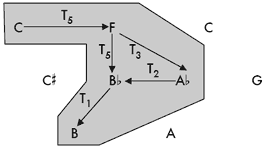

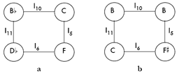
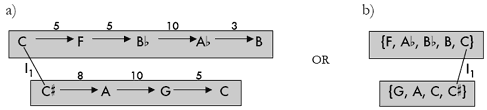
[22] That one T-set is obvious while the other is hidden is purely a product of the way this structure was drawn: i.e., the placement of the nodes and the arrows that Lewin chose to include. There are no rules governing what arrows should be drawn (my S3 might be taken as a commonly abided preference rule—but it is not followed in Figure 7, which, to some degree, accounts for its apparent complexity). In Figure 10, I simplified Lewin’s graphical display to clarify the opposing T-sets. Because all relations within a T-set are transpositional, I omitted the “T” labels in showing the intervallic distances from one pc to another in Figure 10a. I then took the next step of omitting the T-set-internal arrows altogether in Figure 10b. In both Figures 10a and 10b, I labeled only the inversional axis of one token pair of pcs (one pc from each T-set). All other axes can be inferred from this one.(16)
Figure 10. Two simpler displays that more clearly differentiate the two constituent T-sets
(click to enlarge)
Figure 11. Two abstractions, representing all possible K-nets that are positively isographic to Lewin’s rather large K-net
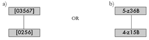
(click to enlarge)
[23] By moving to increasingly abstract levels, we can clarify what is distinct about this entire family of isographic network interpretations.(17) Figure 11 suggests two ways to describe K-net families: the first displays the constituent T-sets in normal form; the second uses names from Forte’s catalog, with the slight variation suggested by Castrén (1994). For inversionally asymmetrical set classes, transpositions of the standard prime form carry the postfix “A” and transpositions of its inversion are labeled “B.” Consider the TnI class [01247] (5-z36): transpositions of [01247] are called 5-z36A and their inversions (transpositions of [03567]) are called 5-z36B. Naturally, any combinations of 5-z36A and 4-z15A can be drawn as negatively isographic to those designs in Figures 7–10.
[24] Recasting K-nets as dual T-sets implicitly obviates the network-internal Tn arrows. As others have mentioned, Tn arrows dynamically model the intervallic relations that are held invariant from one chord to another.(18)
That dynamism is metaphorical in nature (after all, pitches are not literally mapped onto other pitches), but the active language of transformational theory enlivens our analytical narrative. Consider the rhetorical difference between saying “T4 maps A![]() onto C” and “C lies four semitones higher than A
onto C” and “C lies four semitones higher than A![]() ,” or even “the interval between A
,” or even “the interval between A![]() and C is 4 semitones.” However appealing we find the language of transformational theory, its graphical interface often seems a bit ungainly and clarity can be compromised by an abundance of space-consuming graphs that often-unnecessarily interpret every single musical segment.(19)
and C is 4 semitones.” However appealing we find the language of transformational theory, its graphical interface often seems a bit ungainly and clarity can be compromised by an abundance of space-consuming graphs that often-unnecessarily interpret every single musical segment.(19)
Figure 12. Two progressions that feature <T0> relations
(click to enlarge)
Figure 13. Two progressions that feature <T2> relations
(click to enlarge)
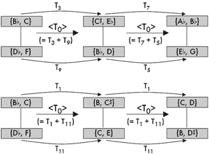
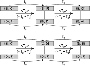
[25] Even the I-arrows, which I have omitted, can be surmised through intervallic analysis. A pattern of increasing or decreasing intervals between the T-sets reflects the degree to which two T-sets maintain constant inversional balance. The distance between internal T-sets can also be inferred from split transformations. If one T-set moves by T2 and the other moves by T11, then clearly the distance between the two T-sets changes by three semitones from one chord to the next.(20) One could even say that inversional balance is more clearly expressed by dual transformation than by network In arrows. Figure 12 illustrates this with two three-network progressions. Each progression maintains <T0> relations from chord to chord, but the split transformations show that only the latter (Figure 12b) truly projects an inversional wedge (or, more accurately, Figure 12b can potentially project a wedge in some musical realizations). Differentiating between these transformational paths seems both worthwhile and simple.
[26] The K-net transformation <T0> means that the (pc space) inversional axis between the two T-sets is maintained from one chord to the next. <T1> signifies that the inversional axis has been offset by one semitone. But <T1> can be realized in many ways. For example, in a two-chord progression, one T-set remains invariant, while the other moves at T1; alternatively, one T-set moves at T2 while the other moves at T11; and so forth. While a case can be made that <T0> transforms maintain a certain degree of consistency (that of inversional balance), what of other <Tn> transforms? Figure 13 shows two progressions that feature <T2> relations. In the first progression (Figure 13a), comparing chords 1:2 with chords 2:3 suggests little similarity of motion. Both are <T2> transforms, but one features T-sets moving by interval classes 5 and 3; the other features motion by ics 4 and 6. However, in the second progression (Figure 13b), a certain consistency is maintained throughout and we can see and potentially hear why this might be called <T2>. The lower T-sets are invariant throughout, while the upper T-sets progressively move at two semitone intervals. Again, K-nets do not differentiate between consistent and inconsistent uses of <Tn> nor do they project the divergent ways in which <Tn> can be calculated.(21)
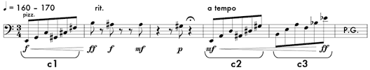
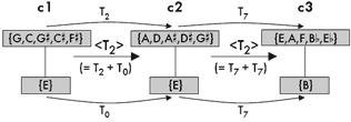
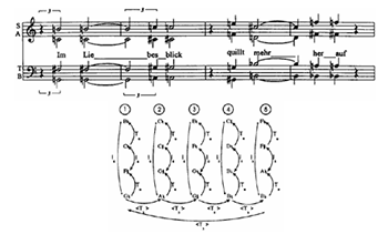
[27] One brief example from the literature will demonstrate a case in which the polyvalence of <Tn> makes K-net isography seem inadequately discriminating. Figure 14 features a brief excerpt from the end of Witold Lutoslawski’s Symphony No. 4 (1992). It is a striking passage for celli alone, one of the few times when only a single instrumental timbre is heard, and it directly follows and precedes moments of complete silence. I will present a K-net-based reading of the three manifestations of the six-note motive (marked c1, c2, and c3), and also make some additional analytical observations.
Figure 14. Lutoslawski, Symphony No. 4, Rehearsal 92, vc. (tutti)
(click to enlarge and listen)
Figure 15. K-net interpretations of the passage from Figure 14
(click to enlarge)
[28] Motives c1, c2, and c3 share the same contour (<013245>) and many intervallic similarities. In fact, when comparing c1 and c2, one would surely notice that, except for the invariant first note, the latter is T2 of the former. Accordingly, in Figure 15, I show a <T2> (T2+T0) K-net transform that resembles the <T2> transformations shown in Figure 13b. By contrast, c2 and c3 belong to the same set class and are, in fact, literal pitch transformations, with the latter lying seven semitones above the former. Using musically consistent segmentation, we can show a T7 relation from the lowest pitch of c2 to the lowest pitch of c3 and another T7 relation from the upper pitches of c2 to the upper pitches of c3. This “split” transformation (T7+T7) combines into another <T2> K-net transform.
[29] Is this musically justifiable? Can we really equate the musical progression from c1 to c2 with that from c2 to c3? Does it make sense to invoke split or K-net transformations when, in fact, the latter pair can be modeled by simple transformations? Intuitively, I want to answer “no” to all these questions despite the fact that Figure 15 is consistent both in the way that it parses the music and in the transformations it shows. In the culture of music analysis, it generally seems desirable to show uniformity wherever possible. There can be little doubt that these three motives are manifestations of the same basic musical gesture, but that musical sameness is not well modeled by <T2>. What c1, c2, and c3 share is intervallic and contour similarity within each motive; what <T2> implies is some similarity in the distance that separates them.
[30] Sometimes, in an effort to consolidate, too much information can be packed into a single number.(22) Because <T2> (or, more generally, <Tn>) can be realized along a wide variety of split transformational paths, I propose a modest elaboration on K-net transformational labels that recognizes their constituent dual transpositions or dual inversions. Rather than merely showing <T2>, I would prefer to stipulate <T2> (0+2), <T2> (7+7), or any of the other possible combinations (there will be six, seven, eleven, or twelve combinations, depending upon whether n is even or odd and whether we choose to differentiate between, say, 0+2 and 2+0). This amendment would allow us to preserve the broad category of K-net hyper-transformation while adding a level of meaning and transparency that would help us understand just what combination of elements led to the <T2> designation. We might even expand our selection of adjectives to include “consistent,” “grand,” or even “super-strong” to describe isographies that maintain the same dual transpositions.
[31] Including such information would surely help anchor this analytical nomenclature a bit more firmly to the musical surface. And, if not treated as merely ancillary data, appending the dual transformational basis of each hyper relationship might well temper, if not assuage, a number of the criticisms found in the next section of this article. An aside: I mentioned earlier that part of transformation theory’s appeal is its apparent dynamism. We often claim that it not only models and compares the contents of particular structures, but rather how it is that we move from one structure to another. (I have again shifted from transformational structuralism to the common metaphor of motion that often drives transformational narrative.) In any case, <Tn> really is a comparison of two internal network structures. It tells us nothing about the path, whereas the specific split transforms do, and they therefore seem more amenable to the often-kinetic language of transformational analysis.
II. Relational Abundance (Promiscuity)
[32] Because any pcset can form multiple K-net interpretations, many pairs of pcsets can be molded into multiple different isographic formations. Indeed, there are far more possible K-net isographies than canonical ways to relate pcsets. This abundance of potential relations could be cast as either a problem (what O’Donnell has deemed “promiscuity”) or a feature, highlighting their inherent flexibility. Inasmuch as K-nets are considered musical interpretations, I am inclined to view their abundant relatability as a good thing. However, when we start talking about K-classes (as does O’Donnell) and especially K-families (as does Lambert) and when the local K-net interpretations do not model salient surface events, I find myself forced to think of them abstractly, in the same basic way as I think about set classes. The operative analytical question shifts from “how can we represent the evident musical voice leading or motivic relationships?” to “can these two pcsets be diagrammed in such a way that they appear isographic?” When I am led to consider the second question, I find relational abundance problematic.
Three-Node K-Nets
[33] Pairs of trichords can be interpreted as isographic K-net structures in numerous ways. If two trichords (or a trichord and a dyad) share even a single interval class, they can be shaped into a pair of isographic networks, and that isography can (willy-nilly) be construed as either positive or negative. As mentioned earlier, an interval can be thought of as a static thing: a distance that simply exists between two notes; or as a dynamic thing: a transformational force that maps one note onto the other. One shared interval translates to one shared Tn arrow, and that is sufficient to draw network isography.[34] We can think of that common interval more generically as a common interval class (rather than a pitch-class interval with range 0–11), since the distance between any two pcs X and Y can be calculated by moving clockwise or counterclockwise along the proverbial pc clock. If it helps to visualize arrows, a single Tn arrow can point from pc X to Y or from Y to X. The distance from X to Y is inversely related to the distance from Y to X, so it follows that drawing negative or positive isography purely reflects an analyst’s discretion and is not inherent to any pair of 3-note pcsets that share an ic.
[35] There are 78 possible pairs of trichords (12+11+10+
Nonetheless, strong, positive, and negative isography have their limitations. Isographically related trichordal K-nets are restricted to collections that share an interval class (ic). For example, since {C, E, G
}, an augmented triad, contains only ic4, it cannot be isographic with {C, C
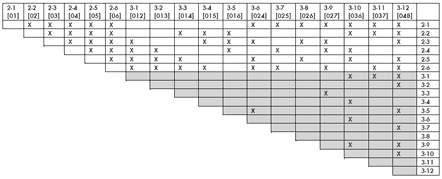
[36] Stoecker (2002) charted all potential trichordal K-net isographies and I have reproduced and expanded his table in my Figure 16, which provides a more detailed view of what is possible when comparing particular dyad- and trichord-classes in three-element networks.(24) The shaded area of this chart clearly shows that not every trichord is equally relatable. [026] can be thought of as something like an all-interval trichord because its elements are separated by one instance of each even ic (2, 4, and 6). Since there are no trichords or larger scs that only include odd ics, once [026] comes to the party, every other trichord enjoys at least one mutual relation.(25) [013], [014], [015], [025], and [037] are almost as promiscuous: each is unrelatable to only a single other trichord. At the other end of the spectrum sits [048] (the uni-interval trichord). But when even it can be isographic with half of its peers, I would suggest that we have a low standard for relatedness.
Figure 16. Trichordal and dyadic set classes that cannot be strong, positively, or negatively isographic with each other
(click to enlarge)
[37] Since the most promiscuous trichord classes include many of the most common and familiar melodic and harmonic structures found in a wide range of repertoire, trichordal isography generally comes easily to those who seek it. When the standard for pcset relatedness is this low, analysts ought to exercise particular diligence and discretion in making a strong case for the uniqueness and musicality of their readings.(26) Though segmentation is not explicitly a topic for this critique, it is only through sensitive segmentation (which must, in turn, rely upon musical parameters other than pc) that three-node K-net analysis can seem compelling. With the addition of O’Donnell’s “double emploi,” by which two different K-net interpretations of a single set allow isography with a pair of otherwise non-isographic K-nets, the standard for relatedness slips further. And with Stoecker’s axial isography, relatedness is even more commonplace.
[38] At this point, it bears repeating that I do not think relational abundance is inherently problematic as long as each relation drawn seems musically motivated. My criticism is therefore aimed at neither Klumpenhouwer’s isography nor Stoecker’s axial isography. Rather, I am skeptical of their use to create overly broad pcset equivalence classes and, especially, of any analytical application founded on the use of such classes.(27)
Larger K-Nets and the Issue of Consistency
Figure 17. Two four-node K-net types (box and umbrella)
(click to enlarge)
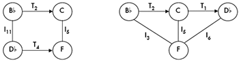
[39] As we move beyond 3-node K-nets, the promiscuity problem is compounded (or perhaps displaced) by the issue of consistency. Four-node networks, for example, can be formatted in two different ways: either like a box, where the two T-arrows bind complementary dyads or like an umbrella, where the two T-arrows bind three notes, omitting a single note. In other words, tetrachords can be split into either a pair of dyadic T-sets or into one trichordal T-set and a singleton. These two configurations are shown in Figure 17.
[40] In published K-net analyses, these two configurations are treated similarly. Using O’Donnell’s double emploi, we could even relate one configuration-type to another. But they are not at all equivalent in relational potential. Think about how common it would be to reach blindly into the bag of all tetrachords and pull out two that shared a pair of non-overlapping interval classes (in this case an ic2 and an ic4) compared with the probability of pulling out two tetrachords that mutually embed a single transpositionally defined trichord class (in this case [023]). Moreover, because isography among box-style 4-node K-nets relies only upon two common ics, such isography can (as with trichordal K-nets) be shown as positive or negative at an analyst’s whim. This is not the case with umbrella-style K-nets.
[41] The standard for K-net relatedness can vary wildly, especially when we interpret larger pcsets, and this seems more troubling than the simple issue of relational abundance. Under such conditions, it can be tough to contextualize your work and discover how significant your analytical claims might be.
On Multiple Interpretations
Figure 18. Dizzy Gillespie, “A Night in Tunisia,” opening gesture split into two four-note segments
(click to enlarge)
Figure 19. Three ways to split α 4-14 {
(click to enlarge)
Figure 20. {

(click to enlarge)
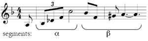
[42] Consider the opening motto of the tune “A Night in Tunisia” by Dizzy Gillespie. The excerpt is shown in Figure 18, divided into two four-note segments marked α and β. Again, isography can be drawn if
α and β are each divisible into two segments {α1,
α2} and {β1, β2} and there are canonical operations that map α1
![]() β1 and α2
β1 and α2
![]() β2. α and β are not wholly related under any individual canonical operation, which is also typical for K-net analysis. Since the canonical operations at play are conventionally transposition and inversion, we can say that while
α and β are not members of the same Tn/TnI sc, they can each be split such that sc(α1) = sc(β1) and sc(α2) = sc(β2).
β2. α and β are not wholly related under any individual canonical operation, which is also typical for K-net analysis. Since the canonical operations at play are conventionally transposition and inversion, we can say that while
α and β are not members of the same Tn/TnI sc, they can each be split such that sc(α1) = sc(β1) and sc(α2) = sc(β2).
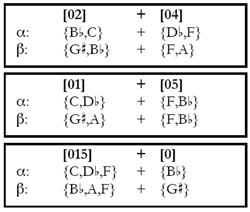
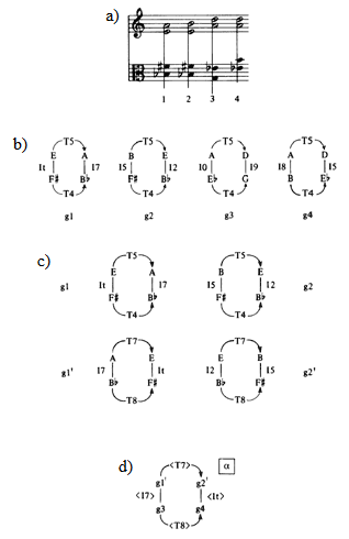
[43] There are three ways in which α, a member of sc 4-14 [0237], and β, a member of 4-4 [0125], can be divided into equivalent sc pairs. Figure 19 displays these partitions and Figure 20 reconfigures them into pairs of isographic K-nets (shown in my preferred dual-transformational orientation), depicting the five possible K-net transformations that map α onto β. As mentioned above, box-style K-nets can be shown to display either positive or negative isography, which is why there are five, not three, possible isographic interpretations.
[44] Taking a tour around Figure 20, I will attempt to provide brief appropriate analytical narratives to substantiate each of these network interpretations. In interpretation I, we could draw out the connection between local T2 arrows that could be inserted in the top T-sets of
α and β and the <T2> transformation between α and β. Finding such correspondences between pc transformations and network transformations is an important step in constructing recursive network structures. (Recursion will be discussed in the last section of this article.) Interpretation II has little potential for recursion, but one could draw attention to the fact that the transformation <I6> finds pc correspondences in the intra-T-set relationships (one in
α {D![]() , F} and one in
β {G
, F} and one in
β {G![]() , B
, B![]() }). Interpretation III can claim a more significant phenomenological connection between pc and network transformations: <T8> might seem more T8-ish because it is formed by a combination of a T0+T8 split (similar to the relationship between c1 and c2 in Figures 14 and 15). Its inversional counterpart, interpretation IV, might be even slightly more impressive in this regard. Both T-sets in
α, members of scs [01] and [05], are inverted in p-space onto the T-sets in β: the <D
}). Interpretation III can claim a more significant phenomenological connection between pc and network transformations: <T8> might seem more T8-ish because it is formed by a combination of a T0+T8 split (similar to the relationship between c1 and c2 in Figures 14 and 15). Its inversional counterpart, interpretation IV, might be even slightly more impressive in this regard. Both T-sets in
α, members of scs [01] and [05], are inverted in p-space onto the T-sets in β: the <D![]() , C> major seventh maps to the
<G
, C> major seventh maps to the
<G![]() ,
A> minor second and the <B
,
A> minor second and the <B![]() up to F> perfect fifth maps to the
up to F> perfect fifth maps to the ![]() down to F> perfect fourth. Finally, interpretation V carries the weight of embedding a mutual trichord class.
down to F> perfect fourth. Finally, interpretation V carries the weight of embedding a mutual trichord class.
[45] How do we make an interpretive decision when faced with these five choices? Do we aim to show consistency between levels of transformation (recursion) or do we try to choose the one that seems most musically appealing? Unfortunately, none of these five choices represents the musical surface very well because each partitions these two segments inconsistently. The [02] dyad (or T2 arrow) spans the first and fourth pcs in α and the first and third pcs in β; the [04] dyad spans the second and third pcs in α and the second and fourth pcs in β; the [01] dyad spans the second and fourth pcs in α and the third and fourth pcs in β; and so forth. It would, in other words, be difficult to attend to the small-scale transformations that any of these networks portrays. When the constituent transformations are relatively abstract, it would be formidable to hear what any of the large-scale isographies represents. Despite this lack of surface support, my earlier analytical statements—at least those about interpretations I, II, and IV—might sound persuasive, especially when coupled with networks that seem so visually appealing.
[46] After the musical surface has been segmented and its fragments have been interpreted as pcsets, networks, or any other abstraction, we often allow ourselves to lose track of the score, almost as if its purpose has been exhausted. This is a danger with any analysis that replaces music notation with non-music symbols, but it is particularly easy to fall into with K-nets, both because the network structures can be shaped and reshaped like modeling clay and also because they inherently require one to focus upon a single parameter. Again, I am advocating neither specificity over generality nor any particular mode of analytical representation. However, I do believe that the more abstract our tools and the greater the potential for relational abundance, the more meticulous we ought to be about demonstrating the musical relevance of our analysis.
[47] Before moving on, it seems worth asking one more question of the analytical interpretations presented above, and it is a question that could rightly be asked of any essentially motivic analysis: why exactly are we trying to relate these two musical segments? They are temporally adjacent, and together they form a motto that is repeated three times during the first six measures of the song, but do they exhibit any common musical features (beyond some shared interval classes) that lead us to consider them as a pair of similar or equivalent motives? If the answer is “no,” is it only our abiding fondness for organicism that drives such motivic analysis?
[48] Contrived examples like the one above allow one to stack the deck a bit, so it seems only fair to bring a published K-net analysis into the critical mix. Henry Klumpenhouwer’s reading of Webern’s Piano Variations, op. 27, mvt. 3, measures 1–12 provides a far more compelling musical analysis than the one I created above.(28) Klumpenhouwer enumerates many network possibilities and two distinct partitional schemes. He invites us to hear and understand this excerpt in multiple ways, yet the analytical paths that he ultimately follows seem to prioritize uniform network (and hypernetwork) structures over motivic consistency.
Figure 21. The opening twelve notes of Webern, opus 23, mvt. 3, segmented into trichords
(click to enlarge)
Figure 22. Six network interpretations of the first trichord (J1 in Figure 20)
(click to enlarge)
Figure 23. One depiction of positive isography among the trichords J1–J4
(click to enlarge)
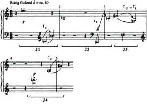
[49] This musical excerpt is a particularly good one for demonstrating the potential value of K-net or split transformational analysis. The first twelve pitches, shown in Figure 21, most obviously divide into four trichords, each featuring two identically articulated tones that span eleven semitones and a third “odd” tone that is articulated differently.(29) (I have drawn these arrows onto Klumpenhouwer’s example.) This twelve-tone movement does not use a derived row. Rather, the four trichords instantiate four different set classes: [015], [012], [013], and [014], respectively. Given this musical scenario, one might expect to see four isographic K-nets, each featuring a single T11 arrow.
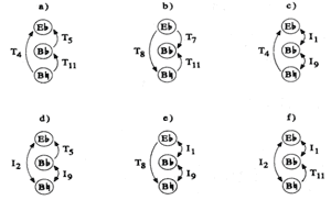
[50] After providing six different well-formed K-net interpretations of the opening three notes (featuring T1, T3, T8, T9, and T11 arrows), Klumpenhouwer ecumenically claims that none of the displayed networks “has inherent analytical value over any other: a given interpretation may be more or less suggestive or useful depending on a particular analytical context.”(30) These six networks are reproduced in Figure 22. While I admire this apparent analytical flexibility and openness, I nevertheless disagree that every interpretation carries musical (much less equivalent musical) potential. It does not seem at all unjust to give priority to those interpretations that noticeably jibe with shared musical features (such as pitch, interval, contour, rhythm, or timbre).
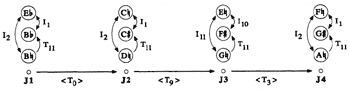
[51] Although Klumpenhouwer does eventually arrive at a network analysis that includes a T11 arrow in each trichordal representation (his Example 14 on p. 30, reprinted as our Figure 23), the second trichord (a member of sc [012]) is partitioned differently than the others, with the T11 arrow drawn between two differently articulated pitches (D and C![]() ). The apparent reason for this re-reading is to show strong isography (<T0>) between the first and second trichords. In this case, it seems that interpretive decisions are steered by a desire to show the sort of unity that K-nets best represent.
). The apparent reason for this re-reading is to show strong isography (<T0>) between the first and second trichords. In this case, it seems that interpretive decisions are steered by a desire to show the sort of unity that K-nets best represent.
[52] In the second half of his article, Klumpenhouwer interestingly re-reads the first twelve notes as segments of 4+5+3 notes. Though his segmentation brings out different (and noteworthy) properties of the row and its musical realization, in producing commensurate (five-node) networks, he interpolates repeated pitch classes in the networks that represent the trichord and the tetrachord. Because there are no repeated pitches or pitch classes among the first twelve notes of the music, these networks compel one to imagine a musical scenario that does not exist. One could argue that repeating pitch classes offers a greater variety of relationships among notes in a musical segment, but that ability is (necessarily) applied inconsistently and arbitrarily. (Klumpenhouwer 1998, 33–37.)
III. The Phenomenology of Displaced Pitch-Class Inversion and Dual Inversion
Figure 24. An example of K-nets that are consistently projected in register
(click to enlarge)
[53] The previous section included a call for some phenomenological grounding when the objects of analysis seem both malleable and distantly removed from the musical surface. When the T-sets that form K-nets are presented in similar registers, timbres, dynamic ranges, etc., K-nets (or dual transformations) can be very compelling. Catherine Nolan presented an exceptionally well-grounded K-net analysis of Webern’s Das Augenlicht, op. 26, at the 2005 Dublin International Conference on Music Analysis. She analyzed the work’s five a cappella choral passages, and in each case where K-nets were used the Tn-arrows were drawn between the upper two voices and also between the lower two voices (in our dual transpositional terms: the T-set pairs were always formed from the SA and TB parts). Moreover, the intervals of transposition were literally projected in p-space, and her graphical display maintained registral integrity. Nolan’s Examples 1a and 1b are reproduced in my Figure 24.
[54] But even in a situation that is this musically clear, I still wonder whether there is much that is T3-like about the <T3> (hyper) transformations that connect all but one pair of adjacent chords in this example. Again, <T3> signifies that T-sets move in a lopsided inversional balance that is skewed by three semitones. But in this case (which is, again, about as musically clear as any example I know), it might be more phenomenologically appealing to depict the progression from chord 1 to 2 as “almost T1” or “almost T2” transpositions in the spirit of Straus’s fuzzy transformations.(31) After all, the entire texture ascends: the top voices by one semitone; the bottom voices by two semitones. On the other hand, the motion between chords 2 and 3 seems more inversion-like since the women’s and men’s parts move in contrary motion. But I again wonder whether one can musically imagine a split T4/T-1 (or T11) transformation as <T3>, and how do we conceive of this <T3> as equivalent to the <T3> (T1/T2 split) that separates chords 1 and 2?
[55] I have no objection to Nolan’s basic analysis, which I find elegant and musically astute. She does not dwell on these displaced inversions, but rather focuses on the dual transpositions. Even so, K-nets (as they have been traditionally drawn) at least implicitly lead one to think about displaced inversion axes. As I mentioned earlier, I suspect that too much information has been packed into a single number and I would rather differentiate these <T3> transformations by highlighting their inherent split transformations: <T3> (1+2) and <T3> (4+11). Of course, doing so (and thereby embracing a “grand isography”) would raise the standard for relatedness, making truly equivalent transformations far more exceptional.
[56] As challenging as it is to construct aural images of displaced pc inversion, as represented by <Tn> transformations, the notion of dual pc inversion implicit in <In> transformations seems far more problematic. Dual pc inversion can be hard enough to hear (or even to imagine hearing) when not realized as musical wedges, and when I think of one part of a chord being transformed by I5 and the other part moving by I8, I can only concede that I would have problems detecting that relation in most musical situations. When we further stipulate that the I5/I8 dual transformation is only one manifestation of the <I1> hyper-transformation, I find myself wondering whether there is any distinctly <I1> (or <In>) sound. Straus vividly encapsulated this problem: “
[57] Of course, I would not want to limit my collection of analytical tools to those that represent things I can always hear. But, again, when various transformations can be used in a single musical situation and, conversely, when single transformations can model a wide variety of musical situations, I do at least want to maintain the possibility of leaning on my own musical sensibilities to select among my options. Otherwise, I fear that my analyses would be modeling neither a composer’s design nor my own musical interpretation.(33)
[58] The K-net literature includes a great many appeals to perception—to “hearing” particular K-net interpretations. Indeed, almost every scholar who has analytically applied K-nets has mentioned audibility, at least in passing.(34) The issue here is not whether K-nets can be used to model an aurally salient passage. Rather, the question I am invariably left asking is whether those salient aspects might more clearly be modeled in some other way. It would be difficult to imagine a situation in which dual transformation did not provide a more straightforward phenomenological account than K-nets.
IV. Hierarchy and Recursion
Figure 25. Four isographic K-nets (g1′, g2′, g3, g4) combine to form a “hyper-network” or “middleground” K-net structure
(click to enlarge)
Figure 26. K-nets intended to reflect the musical surface shown in Figure 25a
(click to enlarge)
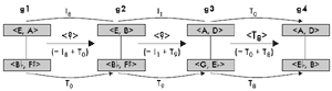
[59] One could avoid the particular phenomenological problem of dual inversion by resolving to employ only positively isographic K-nets, but doing so effectively forfeits one’s ability to produce recursive network structures, and these are perhaps the greatest incentive for using K-nets in the first place. “Recursion,” in the K-net sense, refers to networks of networks, or a grouping of K-nets arranged such that the transformations between selected K-nets mimics the transformations within a single constituent network. Lewin demonstrated recursive network structures and not only made the case for drawing out such hierarchies, but for using them as the basis for selecting among interpretive choices at every level of analysis.(35) Such a recursive structure is shown in Figure 25, which brings together a number of examples from Lewin’s 1994 K-net “tutorial.” Together, these examples illustrate the various stages in moving from surface-level K-nets to deeper-level ones.
[60] Lewin’s textural reduction in Figure 25a clarifies his split-transformational view of this progression from Schoenberg’s, op. 11, no. 2 piano piece. The notes in the upper staff are consistently separated by some manifestation of ic5, and the alto clef notes are consistently separated by some manifestation of ic4. Again, with any pair of invariant interval classes, network isography can be drawn. But how does one decide when, for example, to draw T7 arrows and when to draw T5 arrows? Intuitively, I would probably answer that question in one of two ways: 1) we should call the treble-clef intervals uniformly T5 or uniformly T7 and the alto-clef ones either T4 or T8 (this way is arbitrary, but consistent); or 2) we should try to have our networks reflect the musical surface to the greatest degree possible. Answer #1 reflects Lewin’s initial network drawings, shown in Figure 25b; the latter answer would probably entail a K-net interpretation like that shown in Figure 26, where I have simply replaced Lewin’s and Klumpenhouwer’s nodes with my T-sets. The constituent T-sets are ordered from low to high to reflect Lewin’s musical realizations (though not the actual musical surface). Although this captures Lewin’s musical reduction of this passage, it does not allow isographic relations either from g1 to g2 or from g2 to g3 (although Stoecker’s axial isography would give us a way to relate these chords).(36)
[61] Ultimately, Lewin chooses neither the structural consistency of Figure 25b nor the p-space consistency of Figure 26. His larger purpose in this tutorial was to show hierarchies of network structures and how networks of networks can replicate the design of the their constituents. However, to show these hierarchical “hyper-networks” we need the same distribution of <T> and <I> relations as we have of T and I relations within a single network. Since all K-nets are, by definition, formed by some combination of transposition and inversion, all hyper-networks must comprise both positive and negative isography.
[62] To construct a network of chords g1 through g4 that looks like any of the networks that interprets g1, g2, g3, or g4, Lewin needed to reconfigure two of the chords to form negative isographies. Because he uses the box—not the umbrella—configuration, both dyads within a network can be flipped to construct mirror-image K-nets. As mentioned in the section on relational abundance, any four-node box-style (#2+#2) K-net can be reconfigured to form its own inversion. Figure 25c compares g1 and g2 to their inversional doppelgangers, g1′ and g2′. (Again, it is only the graphs, not the pcsets, that are inversionally related.) A final hyper-network that interprets g1′, g2′, g3, and g4 in a way that is strongly isographic with g1′ is shown in Figure 25d.(37)
[63] One reason that I admire Catherine Nolan’s analysis (reproduced in Figure 24 above) is that she used K-nets without drawing out recursive relations. Indeed, her networks could not be placed into a hyper-network without reconfiguring some of the local structures in ways that obscure their p-space realizations. Forming recursive K-net structures would not only be arbitrary in such an instance, it would necessarily represent weaker musical relationships than actually exist. This circumstance hardly seems extraordinary. Rather, I have trouble imagining instances in which recursive K-net structures would portray stronger relationships (at least experientially) than would K-nets related exclusively by <Tn>.
[64] At the beginning of this article, I quoted Straus’s comment that recursion is only problematic “when our desire for it leads us to emphasize musical features that might otherwise be of relatively little interest.”(38) But there are more frustrating and systemic problems with recursion than the unpleasant by-product Straus mentioned. Recursive analysis requires us to locate positive and negative surface-level isographies in the same quantity as shown in any one local K-net. This often entails skewing surface readings into representations that simply provide the right type of graph to fit the situation.
[65] A more pragmatic problem that arises when constructing K-net superstructures is that K-nets of size q must be grouped into q-sized hyper-networks for recursion to be drawn. Extended outward, q-sized K-nets must form into hyper-networks of size qn, where n is an integer that reflects the recursive level and “size” refers to the number of pcs in the network or hyper-network. There are not many musical situations where q-note chords cluster into q-chord progressions (and q progressions of progressions, and so on). Therefore, musicians who choose to frame their analyses around hyper-networks are often left with the choice of selectively omitting some chords or reusing some chords in other structures.(39) And, of course, all chords need to contain the same number of notes or else some notes need to be duplicated within a surface K-net, since no one has yet suggested a way of relating different sizes of networks.(40)
[66] But still a larger problem with K-net recursion has to do with what it inherently shows. Lewin and others have compared hyper-networks and hyper-hyper-networks to the levels in a Schenkerian analysis. Though Lewin admits that this similarity is structural and not phenomenological, likening network and Schenkerian levels is misleading.(41) Every level of a Schenkerian analysis (except, perhaps, the ultimate “chord of nature”) relates the same sorts of objects. A tone and/or harmony found on the middleground should be present (or at least be implicit) on every shallower level, and every level of a Schenkerian analysis details tonal and contrapuntal relationships. K-net hierarchies yield no such consistency. The objects of a “foreground” K-net are (generally) pitch classes and the transformations that map those pitch classes to each other; the objects of a “middleground” K-net are transformations and the transformations that map those transformations to each other. At every level other than the “foreground,” K-nets interpret increasingly abstract relationships of relationships, not relationships of notes or pitch classes. In Schenkerian analysis, notes are present at every level and pitch structures are never replaced by relational structures.
[67] This flawed analogy, however, seems less troubling than the more primary supposition that K-nets group into meaningful hierarchies. O’Donnell also expressed this in his dissertation, calling the levels “non-hierarchical because they model different aspects of the music, and one interpretation does not subsume the next as in a Schenkerian graph.”(42) This is why I disagree with Lewin that hyper-networks can provide a compelling rationale for interpreting surface structures. For that matter, I think that persuasive Schenkerian analyses generally do not (and should not) use middleground evidence to support and arrive at foreground decisions. Such top-down approaches to analysis often lead us to find only that for which we are looking.
[68] For all the structural elegance of recursive networks, they force analysts to abide by quite a few arbitrary limitations. These include the number of networks that can be related in a particular setting and the quality and variety of transformations that may be included in those settings. Although there are numerous ways to draw any particular K-net, and that flexibility makes it relatively easy to generate local isographies, when we start building hyper-network structures, we also force ourselves to designate a single K-net as the sort of mother network, and that priority does not need to be grounded in musical salience. That, combined with the musical incommensurability of upper- and lower-level structures, is why I find recursion unconvincing and even potentially detrimental. In the first section of this article, I proposed redrawing local K-nets as dual transformations and dropping the internal I-arrows that point from one T-set to the other. I mentioned that the sole consequence of this simplification would be losing the possibility for recursive network analysis. It should now be evident that I find that loss to be unproblematic.
[69] It seems to me that the greatest strength of K-nets and also of dual or near transformations lies in their ability to model a common musical situation: that of divergent motion in a polyphonic space. Although hyper transposition is a useful addition to our canon of transformational descriptors, it does not uniquely rely upon the K-net design. We all have different goals for analysis, but surely one central purpose is to clarify and explain. There may not be any inherently easy ways to model difficult music; I just want to be certain that my analytical tools help me elucidate more complexities than they introduce. That might be the simplest and best reason to reconsider Klumpenhouwer networks.
Michael H. Buchler
Florida State University
College of Music
Tallahassee, FL 32306-1180
mbuchler@fsu.edu
Works Cited
Benjamin, William. 1974. Review of Allen Forte’s The Structure of Atonal Music. Perspectives of New Music 13, no. 1: 170–190.
Berry, Michael. 2005. “Josef Matthias Hauer’s Nachklangstudie, Op. 16, No. IV: K-nets Outside the Mod 12 Universe.” Paper presented at the Dublin International Conference on Music Analysis, Dublin, Ireland.
Brown, Stephen. 2003. “Dual Interval Space in Twentieth-Century Music.” Music Theory Spectrum 25, no. 1: 35–57.
Buchler, Michael. 2000. “Broken and Unbroken Interval Cycles and their use in Determining Pitch-Class Set Resemblance.” Perspectives of New Music 38, no. 2: 52–87.
—————. 2001. “Relative Saturation of Intervals and Set Classes: A New Approach to Complementation and Pcset Similarity.” Journal of Music Theory 45, no. 2: 263–343.
Castrén, Marcus. 1994. RECREL: A Similarity Measure for Set-Classes. Studia Musica 4. Helsinki: Sibelius Academy.
Cohn, Richard. 1988. “Inversional Symmetry and Transpositional Combination in Bartók.” Music Theory Spectrum 12: 19–42.
Forte, Allen. 1973. The Structure of Atonal Music. New Haven: Yale University Press.
Gollin, Edward. 1998. “Some Unusual Transformations in Bartók’s ‘Minor Seconds, Major Seconds’.” Intégral 12: 25–51.
Headlam, Dave. 2002. “Perle’s Cyclic Sets and Klumpenhouwer Networks: A Response.” Music Theory Spectrum 24, no. 2: 246–256.
Klumpenhouwer, Henry. 1991a. “Aspects of Row Structure and Harmony in Martino’s Impromptu Number 6.” Perspectives of New Music 29: 318–54.
—————. 1991b. “A Generalized Model of Voice-Leading for Atonal Music.” Ph.D. dissertation, Harvard University.
—————. 1994. “An Instance of Parapraxis in the Gavotte of Schoenberg’s Opus 25.” Journal of Music Theory 38: 217–48.
—————. 1998a. “The Inner and Outer Automorphisms of Pitch-Class Inversion and Transposition: Some Implications for Analysis with Klumpenhouwer Networks.” Intégral 12: 81–93.
—————. 1998b. “Network Analysis and Webern’s Opus 27/III.” Tijdschrift voor Muziektheorie 3, no. 1: 24–37.
Lakoff, George and Mark Johnson. 1980. Metaphors We Live By. Chicago: University of Chicago Press.
Lambert, Philip. 2002. “Isographies and Some Klumpenhouwer Networks They Involve.” Music Theory Spectrum 24, no. 2: 165–195.
Lerdahl, Fred and Ray Jackendoff. 1983. A Generative Theory of Tonal Music. Cambridge, MA: MIT Press.
Lewin, David. 1982–83. “Transformational Techniques in Atonal and Other Music Theories.” Perspectives of New Music 21: 312–71.
—————. 1987. Generalized Musical Intervals and Transformations. New Haven: Yale University Press.
—————. 1990. “Klumpenhouwer Networks and Some Isographies That Involve Them.” Music Theory Spectrum 12: 83–120.
—————. 1993. Musical Form and Transformation: 4 Analytic Essays. New Haven: Yale University Press.
—————. 1994. “A Tutorial on Klumpenhouwer Networks, Using the Chorale in Schoenberg’s Opus 11, No. 2.” Journal of Music Theory 38: 79–101.
—————. 2002. “Thoughts on Klumpenhouwer Networks and Perle-Lansky Cycles.” Music Theory Spectrum 24, no. 2: 196–230.
Losada, Catherine. 2000. “Klumpenhouwer Networks as Determinants of Structural Recurrence at Different Hierarchical Levels: A Critical Approach.” Unpublished ms.
Mead, Andrew W. 1984. “Pedagogically Speaking: A Practical Method for Dealing with Unordered Pitch-Class Collections.” In Theory Only 7, nos. 5–6: 54–66.
Morris, Robert D. 1982. “Set Groups, Complementation, and Mappings among Pitch-Class Sets.” Journal of Music Theory 26, no. 1: 101–144.
—————. 1987. Composition with Pitch Classes. New Haven: Yale University Press.
—————. 1998. “Voice-Leading Spaces.” Music Theory Spectrum 20: 175–208.
Nolan, Catherine. 2005. “More Than Meets The Eye: Text, Texture and Transformation in Webern’s Das Augenlicht, Op. 26.” Paper presented at the Dublin International Conference on Music Analysis, Dublin, Ireland.
O’Donnell, Shaugn. 1997. “Transformational Voice Leading in Atonal Music.” Ph.D. dissertation, City University of New York.
—————. 1998. “Klumpenhouwer Networks, Isography, and the Molecular Metaphor.” Intégral. 12: 53–80.
—————. 2005. “If-Only Networks and Analytical Desire.” Paper presented at the Dublin International Conference on Music Analysis, Dublin, Ireland.
Stoecker, Philip. 2002. “Klumpenhouwer Networks, Trichords, and Axial Isography.” Music Theory Spectrum 24, no. 2: 231–245.
Straus, Joseph N. 2003a. “Uniformity, Balance, and Smoothness in Atonal Voice Leading.” Music Theory Spectrum 25, no. 2: 305–352.
Straus, Joseph N. 2003b. “Three Problems in Transformational Theory.” Talk delivered at the closing plenary session of the Mannes Institute on Transformational Theory, New York City, NY.
Vishio, Anton. 1991. “An Investigation of Structure and Experience in Martino Space.” Perspectives of New Music 29, no. 2: 440–476.
Footnotes
1. Arguably, they have seen even more use than the more straightforward network structures Lewin described and demonstrated in
Generalized Musical Intervals and Transformations (1987) and Musical Form and Transformation: 4 Analytic Essays
(1993).
Return to text
2. Here, and throughout this article, “chord” is used in
the most generic way possible, as a synonym of “set” or “klang.”
Return to text
3. In some ways, the present essay is quite loosely modeled after William Benjamin’s insightful 1974 review of Allen Forte’s The Structure of Atonal Music. (Perspectives of New Music 13:1, 170–190.) Unlike Benjamin, however, I am not critiquing one person’s work. Rather, I draw upon the broadening K-net literature listed among my references.
Benjamin structured his review around six fundamental criticisms:
“I. The Problem of Segmentation
II. The Problems of Derivation and Order
III. The Problem of Context
IV.
Neglected Aspects of Pitch-class and Pitch Structure
V. The Problem of
Explanation
VI. The Significance of the Set-complex.” (177)
Many of Benjamin’s
thirty-year-old criticisms can likewise be applied to K-net usage. Although this
article raises different issues (and also raises issues differently), many of
Benjamin’s thoughtful lines of reasoning have inspired my own arguments.
Return to text
4. Straus 2003.
Return to text
5. As I was preparing my article for publication, one of MTO’s anonymous readers brought to my attention an unpublished manuscript by Catherine Losada (2000). Losada kindly shared her work with me and I have tried to cite it in cases where we have made common arguments. She is preparing a response to my article that will, I hope, bring many of her own strong K-net criticisms to the fore.
Return to text
6. See S1, comment 1.2. One possible substitute for pc inversion is the circle of fourth and fifth transforms (M5 and M7). However, since this article aims to critique K-nets as they have been used (rather than how they might be used), I will not explore such alternatives herein.
Return to text
7. O’Donnell calls these “Lewin networks” or “L-nets” (O’Donnell 1998, 53.)
Return to text
8. The ensuing discussion of Figures 7 through 11 will further demonstrate the necessity for understanding implicit relations.
Return to text
9. However, In arrows are defining aspects of Stoecker’s “axial isography” (Stoecker 2002).
Return to text
10. Losada also makes this observation. (Losada 2000, 19.)
Return to text
11. Following a clear, if slightly inelegant, convention, I am referring to the values of the Tn and In arrows. In fact, such statements should be understood to mean the value of n. This corollary might be more clearly, if clumsily, rewritten as follows: When the respective values of n are identical in two K-nets’ Tn arrows, but their respective Im arrows reflect different inversional axes, the respective values for
m will always differ by a constant value.
Return to text
12. More specifically, the number of distinct ways to partition an n-sized collection into T-set pairs = 2n-1 – 1. E.g., where n = 3, elements {a, b, c} can be arranged into three partitions (22 – 1): ab+c, ac+b, and bc+a. Where n = 4, elements {a, b, c, d} can be arranged into seven partitions (23 – 1): a+bcd, b+acd, c+abd, d+abc, ab+cd, ac+bd, and ad+bc. 5-note collections can be drawn as K-nets in 15 distinct ways, 6-note collections can be drawn as K-nets in 31 distinct ways, and so forth. By “distinct,” I mean distinct pairs of (unordered) T-sets that fall out of any given K-net, not the number of specific orientations of nodes and arrows (a far greater value). As such, ab+cd, ba+cd, ab+dc, and ba+dc are all manifestations of a single distinct partition.
Return to text
13. This observation does not originate with this article. O’Donnell introduced the notion of “dual transformations” in his dissertation, wherein he also made the observation that his and Klumpenhouwer’s models described the same phenomenon, but that the latter “disguises the parsing with its unified graphic representation.” (O’Donnell, 48.) Earlier, Lewin implicitly said the same thing when he, citing Klumpenhouwer, mentioned that isography can be attained in any pair of sets of size n that either share a subset of size n-1 or share two complementary T-sets. (Lewin 1990, 90.)
Return to text
14. For simplicity, the graphed pcs are no longer encircled.
Return to text
15. Lewin takes a different path to arrive at the same pair of T-sets. See his Figures 6.3 and 6.4 and the text on pp. 215–217 in Lewin 2002.
Return to text
16. As such, my Figure 10 somewhat resembles Lewin’s Figure 6.6a (Lewin 2002), which isolates the same two pc collections.
Return to text
17. O’Donnell classifies the set of all positively and negatively isographic K-nets as a “K-net family.” O’Donnell 1998 (72-4) and Lambert 2002 provide detailed elaborations on and enumerations of K-net families, particularly among three-node networks. Members of a particular family are any K-nets (or the pcsets they interpret) that are formed by transposing or inverting both constituent T-sets.
Return to text
18. Dmitri Tymoczko made this point quite lucidly, if informally, in a letter to smt-talk (Re: [Smt-talk] Dogmas 3,4 - GIS - Interval fields.
Smt-talk listserve: Wed, 24 Aug 2005.). Others who have equated (or at least equivalenced) transposition arrows and intervallic labels or dyad classes within the context of K-nets include Lewin 1990 (89), Gollin 1998 (40), Stoecker 2002 (233), Lambert 2002 (170), and Brown 2003 (47).
Return to text
19. This practical concern resembles that faced by analysts who syntactically diagram large tonal works using the methodology enumerated by Lerdahl and Jackendoff in
A Generative Theory of Tonal Music (1983).
Return to text
20. I have claimed that both the network-internal Tn and In arrows can effectively be replaced with intervallic and/or T-set class designations. One might reasonably protest that while the Tn and In arrows seem a bit pedantic at the surface, they are crucial in drawing recursive transformations that mimic the “foreground” networks. This objection will be discussed in section IV of this article (on hierarchy and recursion).
Return to text
21. O’Donnell (1998) makes a similar claim. After illustrating how split transformations T3/T9 can be combined to produce the K-net transformation <T0>, which masks any dual musical motion, he comments: “Most significantly, the precise linear transformation is irrelevant; the only requirement is that the two hands travel the same distance. In fact, c1
![]() c1 is as much <T0> as c1
c1 is as much <T0> as c1
![]() c2" (70).
c2" (70).
Stephen Brown’s (2003) “dual interval space” (DIS)
provides an altogether different, if complementary, way of relating chords that
share two interval classes. For situations like those shown in the four-node
(2+2) K-nets in Figures 4, 5, 6, 12, and 13, his model arguably provides a more
meaningful distance measurement than K-net transformations, though it is less
universally applicable.
Return to text
22. To be both fair and consistent, this same criticism could justly be leveled against my own earlier work on similarity relations (Buchler 2000, 2001).
Return to text
23. It should be noted, however, that Stoecker only advocated using axial isography when the musical surface suggested drawing such relations, not as an abstract prototype.
Return to text
24. The comparison of #3 to #2 pcsets is possible when one pc in the dyad is shown twice in the network. Though such networks imply the presence of two pitch realizations of that duplicated pc (i.e., a multiset), the duplicate pc is often present only in the analysis for the sake of relating different-sized sets.
An anonymous reader of this article pointed out a particularly disturbing consequence of arbitrarily double-counting a single pc for the sake of comparing dyads to trichords: one could likewise double-count elements in two dyads, thereby comparing, for example, an instance of [03] to one of [04]. In such a situation, one would only need to show mutual T0 arrows in each three-element dyad-class. Were we to adopt this standard (and the rationale for relating dyads to trichords strongly suggests that we do so), any dyad could be isographic to any other dyad, and the chart of impossible isographies in Figure 16 would seem even more barren.
Return to text
25. [026] is also embedded in nine of the 28 tetrachord classes, including the two all-interval tetrachords. There are no other trichord classes that are embedded in as many as or more than nine tetrachord classes.
Return to text
26. Catherine Losada (2000) also argued for similar conditions for K-net “significance.”
Return to text
27. For instance, Michael Berry employed K-nets in a mod-7 space to interpret a composition by Hauer. Berry limited himself to trichordal segments, and he worked entirely within pc space. In mod-7 pc space, there are only three interval classes (not including ic0) and four trichord-classes: [012], [013], [014], and [024]. Mod 7 [013] includes instances of all three interval classes; the other three trichord classes each exclude only a single ic. Because in this space no pair of trichords can feature mutually exclusive interval content, every pair of mod-7 trichords can be related by K-net isography, and most pairs can be related in multiple ways. Moreover, Berry used O’Donnell’s “double emploi” which, in mod 7 space, ensures that in any progression of sets, each pair can be interpreted as positively isographic. When isography (or any other sort of relation) is guaranteed, one could just as well say that nothing is particularly related to anything else. (Berry 2005.)
Return to text
28. Klumpenhouwer 1998b. An earlier version of this analysis appeared in Klumpenhouwer’s (1991b) dissertation.
Return to text
29. More accurately, the second trichord features a 23-semitone leap (from C![]() 2 to C4).
2 to C4).
Return to text
30. Klumpenhouwer 1998b, 27.
Return to text
31. Straus 2003a.
Return to text
32. Straus 2003b. Losada likewise describes the problems of inversional relationships at different, and increasingly abstract, levels of structure. She also compellingly problematizes the use of index numbers both locally and hierarchically. (Losada 2000, 16–19.)
Return to text
33. Vishio (1991) combines pc- and p-space to provide especially compelling network analyses that maintain relatively close ties to the musical surface in his analysis of the first Fantasy from Martino’s
Fantasies and Impromptus.
Return to text
34. Lewin’s expository article on K-nets includes a lengthy section on phenomenology. In his afterword, he comments: “Initially skeptical about the analytic significance of Klumpenhouwer’s Networks, I soon became drawn into their study myself, and enthusiastic about their potential. To some extent my conversion involved working out in my own terms a phenomenology to support the implicit analytic assertions of the Networks.” (Lewin 1990, 115.) Other articles that appeal to how we might hear K-nets interpretations include Lewin 1994 (79–86, 98–99), Klumpenhouwer 1998a (91–3) and 1998b (24–6, 31–3), Vishio 1991, O’Donnell 1997 (71–2), 1998 (70), and 2005, Lambert 2002 (168–9 and 178–81), and Stoecker 2002 (236–9). Many more examples can be found; I arbitrarily limited this list to items already in the article’s bibliography.
Return to text
35. Indeed, Lewin clarified that “the recursive potentialities of the theoretical apparatus” was his contribution, not Klumpenhouwer’s. (Lewin 1990, 115.)
Return to text
36. Again, Stoecker only advocated using axial isography when the surface of the music suggested drawing such relations. Lewin’s reduction (shown in Figure 25a) uses different clefs and noteheads (open and filled) to create segments that are not obvious in the score.
Return to text
37. The graph in Figure 25d is only marginally different from the one Lewin produced in his Example 13 (Lewin 1994, 90). His hyper-network connects g1, g2, g3', and g4' in a manner that is strongly isographic with g1'. I preferred explicitly including the model network (g1') in the hyper-network.
Return to text
38. Straus 2003b.
Return to text
39. Lewin (1994) chooses both options in his analysis of the chorale from Schoenberg’s Opus 11, No. 2. In his Ex. 14 (p. 91), he interprets chords 4, 5, 7, and 8 (omitting 6); in Ex. 15 (also p. 91), he shows two networks, interpreting chords 8, 9, 10, 11 and then 10, 11, 12, 13 (overlapping 10 and 11).
Return to text
40. As mentioned earlier, Klumpenhouwer (1998b) does relate a 5-note pcset to a 4-note pcset to a 3-note pcset, but he needs to use entirely 5-node (2+3) K-nets in so doing. This means arbitrarily duplicating one pc in one of his networks, and two pcs in another network. One essential problem with doing this is that the dyadic T-set in his 3+2 split is fully embedded in its companion trichordal T-set. The doubly interpreted pcs are not repeated on the musical surface. (Klumpenhouwer 1998b, 33–35.)
Return to text
41. Lewin wrote: “When a lower-level Klumpenhouwer Network
is interpreting a chord, and a higher-level network-of-networks is interpreting
a progression of chords (more precisely, of chord-interpretations), I noted that
one could conceive of the higher-level network as “prolonging” the lower-level
one, particularly when the given chord is part of the given progression. This
potentiality of the system, observed again and again in the article, can afford
an especially compelling rationale (albeit a non-phenomenological one) for
asserting one particular Klumpenhouwer Network rather than another, to interpret
a given chord. I found it suggestively comparable, methodologically, to the ways
in which a choice among foreground readings in a Schenkerian analysis can be
influenced by middleground considerations.” (Lewin 1990, 115.)
Return to text
42. Backing away slightly, O’Donnell continued: “They do, however, suggest varying degrees of distance from the musical surface, or varying locations on the concrete
![]() abstract continuum.” (O’Donnell 1997, 66–67.)
abstract continuum.” (O’Donnell 1997, 66–67.)
Return to text
Benjamin structured his review around six fundamental criticisms:
“I. The Problem of Segmentation
II. The Problems of Derivation and Order
III. The Problem of Context
IV.
Neglected Aspects of Pitch-class and Pitch Structure
V. The Problem of
Explanation
VI. The Significance of the Set-complex.” (177)
Many of Benjamin’s thirty-year-old criticisms can likewise be applied to K-net usage. Although this article raises different issues (and also raises issues differently), many of Benjamin’s thoughtful lines of reasoning have inspired my own arguments.
Stephen Brown’s (2003) “dual interval space” (DIS) provides an altogether different, if complementary, way of relating chords that share two interval classes. For situations like those shown in the four-node (2+2) K-nets in Figures 4, 5, 6, 12, and 13, his model arguably provides a more meaningful distance measurement than K-net transformations, though it is less universally applicable.
An anonymous reader of this article pointed out a particularly disturbing consequence of arbitrarily double-counting a single pc for the sake of comparing dyads to trichords: one could likewise double-count elements in two dyads, thereby comparing, for example, an instance of [03] to one of [04]. In such a situation, one would only need to show mutual T0 arrows in each three-element dyad-class. Were we to adopt this standard (and the rationale for relating dyads to trichords strongly suggests that we do so), any dyad could be isographic to any other dyad, and the chart of impossible isographies in Figure 16 would seem even more barren.
Copyright Statement
Copyright © 2007 by the Society for Music Theory. All rights reserved.
[1] Copyrights for individual items published in Music Theory Online (MTO) are held by their authors. Items appearing in MTO may be saved and stored in electronic or paper form, and may be shared among individuals for purposes of scholarly research or discussion, but may not be republished in any form, electronic or print, without prior, written permission from the author(s), and advance notification of the editors of MTO.
[2] Any redistributed form of items published in MTO must include the following information in a form appropriate to the medium in which the items are to appear:
This item appeared in Music Theory Online in [VOLUME #, ISSUE #] on [DAY/MONTH/YEAR]. It was authored by [FULL NAME, EMAIL ADDRESS], with whose written permission it is reprinted here.
[3] Libraries may archive issues of MTO in electronic or paper form for public access so long as each issue is stored in its entirety, and no access fee is charged. Exceptions to these requirements must be approved in writing by the editors of MTO, who will act in accordance with the decisions of the Society for Music Theory.
This document and all portions thereof are protected by U.S. and international copyright laws. Material contained herein may be copied and/or distributed for research purposes only.

Prepared by Brent Yorgason, Managing Editor and Tahirih Motazedian, Editorial Assistant